
Key Takeaways
- Cycle count is a symptom, not the definition — LCF is defined by macroscopic plastic deformation in every cycle, so local yielding puts you in LCF territory whether the design life is 400 cycles or 40,000.
- The hysteresis loop evolves before it settles — cyclic hardening or softening shifts the loop over the first cycles, so strain ranges must come from the stabilized response, never the first cycle.
- Coffin-Manson is empirical, not mechanistic — it links plastic strain amplitude to life reliably, but has no fatigue limit and needs four material constants once the elastic term is added.
- Mean stress largely relaxes away in deep LCF — plastic shake-down drives it toward zero, so corrections matter most in the transition band and at longer lives.
- Kinematic hardening is mandatory, calibrated on cyclic data — isotropic hardening misses the Bauschinger effect, and monotonic curves misrepresent a cyclically softening material entirely.
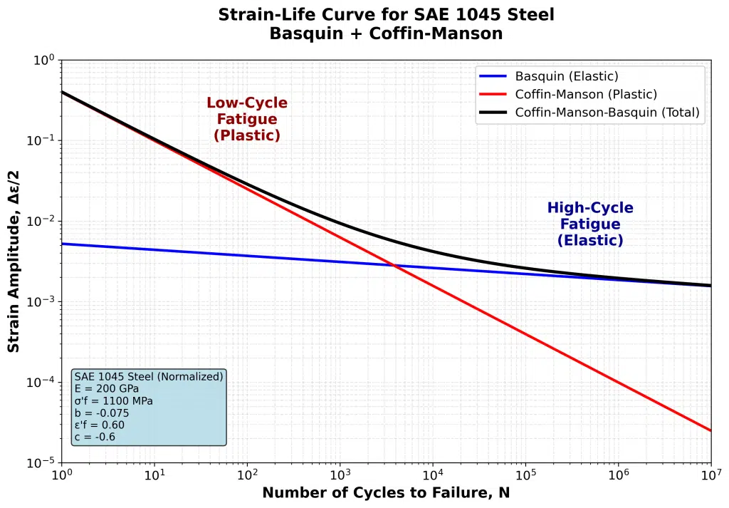
Table of Contents
When your FEA results show stresses above yield and your S-N based life predictions start diverging wildly from test data, you are almost certainly looking at low cycle fatigue — the failure mode behind turbine disk cracking in aerospace and pressure vessel ruptures in petrochemical plants. The difficulty is rarely in spotting that something is wrong. It is in correctly capturing the plastic deformation that drives the damage, and converting that into a life prediction you can defend.
This guide covers the theory, the calculation route, and the FEA implementation strategy you need to handle LCF with confidence — the mechanisms that separate LCF from elastic fatigue, the Coffin-Manson methodology for calculating cycles to failure, mean stress treated properly, and a practical simulation workflow.
What is low cycle fatigue?
Low cycle fatigue (LCF) is a fatigue failure mechanism in which the applied load drives the material past its yield strength, so that measurable plastic strain is produced on every cycle. Failure typically arrives somewhere between 10² and 10⁴ cycles, with the plastic component of strain — not the elastic one — controlling the rate of damage accumulation. That is the fundamental split from high cycle fatigue, where the material stays essentially elastic on a macro scale and damage takes millions of cycles to build.
The boundary is widely misunderstood, so it is worth being precise: cycle count is a symptom, not the definition. The transition between low and high cycle fatigue is not fixed at any particular number of cycles. The meaningful distinction is that LCF involves macroscopic plastic deformation in each cycle, while HCF is macroscopically elastic. If your component yields locally on every load application, you are doing LCF analysis — whether the design life is 400 cycles or 40,000.
The Role of Plastic Strain in LCF Failure
In the elastic regime, stress and strain are locked together by the elastic modulus, which is exactly why stress-based methods work so well for HCF: knowing one tells you the other. Once the material yields, that one-to-one link breaks. Load and unload a specimen past yield and the stress-strain path no longer retraces itself — it opens into a hysteresis loop. The area enclosed by that loop is energy dissipated irreversibly in the material on each cycle, and it is the mechanical signature of the damage process.
Inside the material this is dislocation activity on a scale elastic cycling never produces. Reversed plastic flow moves and multiplies dislocations, concentrates slip into persistent slip bands, and roughens the free surface until microcracks nucleate — and under LCF conditions it happens fast. Small cracks form almost immediately, and because the stress is so high, final fracture arrives while those cracks are still short. There is barely any period of detectable crack growth, which matters for life management: damage-tolerance thinking, built on catching a crack and tracking it, has very little room to operate here.
One asymmetry deserves particular attention: after plastic deformation in tension, the yield strength on the subsequent compression reversal is reduced — the Bauschinger effect. Any cyclic plasticity model you use has to reproduce this, or your hysteresis loop will be the wrong shape and your strain range wrong with it.
💡 Pro Tip: When screening FEA results for LCF conditions, peak stress is not the indicator to look at. Check whether equivalent plastic strain (PEEQ in Abaqus, EPEQ in Ansys) is increasing cycle over cycle. Non-zero plastic strain accumulating on each reversal is your signal that stress-life methods no longer apply.

Cyclic Hardening, Softening, and Why the Stabilized Loop Matters
This is the mechanism most often skipped in introductory treatments, and the one that determines whether your numbers mean anything. The hysteresis loop is not a fixed object. Its shape evolves over the first cycles, and the direction it evolves depends on the material’s prior condition. Under constant strain amplitude cycling there are two opposite behaviours:
- Cyclic strain hardening. The stress needed to enforce the same strain amplitude climbs cycle after cycle. Typical of initially soft materials, where there is capacity for dislocation structures to build up.
- Cyclic strain softening. The same strain amplitude is sustained by a progressively lower stress. This appears in materials already hardened before the test, by heat treatment or cold work. Cyclic plasticity rearranges the strained microstructure, releasing some of the stored energy in the matrix, and the material effectively gets softer.
Either way the transient dies out, stabilizing at a steady loop after a number of cycles that is normally small relative to total life. How quickly is material-dependent: several heat-treated high-strength alloys are near-stable almost from the first cycle, while soft materials and materials hardened by deformation processing are far less predictable.

A companion effect explains why LCF is studied under strain control in the first place. Cycle at constant stress amplitude with Smax above yield and the first upload produces a large plastic excursion — but the unload and reload that follow produce a much smaller plastic strain amplitude, because the material has strain hardened. The loop shrinks and can then be sustained for many cycles. Constant strain cycling removes that escape route: the amplitude is imposed and held, so the material must keep deforming plastically. That is both more severe and a closer match to real structures, where thermal mismatch or stiff surrounding structure imposes displacement rather than force.
⚠️ Common Mistake: Extracting the plastic strain range from the first cycle. The first loop is a transient and is not representative of anything. Always take the range from the stabilized response — conventionally at half-life, or once the loop shape has converged in your analysis.
Identifying LCF Loading Conditions in Engineering Applications
LCF becomes the governing design case when a structure sees only a modest number of load cycles over its economic life. Insisting that every stress stay under the fatigue limit in that situation buys you a structure that is much heavier than it needs to be, for no benefit. Two examples make the point: a vessel that sees pressurization only a handful of times across many years of service, and power generation equipment running hot where the count of on/off transitions is genuinely low.
That second example carries the more important lesson. When stresses arise from differential thermal expansion, the loading is fundamentally strain-imposed, not stress-imposed — a constrained hot region cannot choose how much it expands. This is why thermal cycling problems belong in the strain-life framework almost by definition, and why treating them with an S-N curve is not a conservative simplification but a category error.
Typical situations that put you in LCF territory: startup and shutdown transients in turbines, boilers and reactors; pressure cycling in vessels and piping with a low cycle count over design life; centrifugal load changes tied to operating cycles; thermal gradients across engine blocks, cylinder heads and combustor liners; and seismic or extreme-event loading in structural steelwork.
Low Cycle Fatigue vs. High Cycle Fatigue: Critical Differences for Analysis
The two regimes differ in which strain component dominates, and that single difference propagates through every downstream choice in your analysis. Choosing the wrong framework is not an academic error — it produces life predictions that are non-conservative in exactly the situations where you can least afford it.
Strain-Life vs. Stress-Life Approaches
There is a neat piece of evidence for why strain is the right control variable at short lives. An S-N curve has two horizontal asymptotes: the fatigue limit at the bottom, and an upper one near the tensile strength, where the specimen fails on the first load application. That upper asymptote disappears when the same data is replotted against strain amplitude — the ε-N curve stays linear on log-log axes right down into the very low cycle range. Strong evidence that strain, not stress, is what the material responds to once it is deforming plastically.
| Parameter | Low Cycle Fatigue (LCF) | High Cycle Fatigue (HCF) |
|---|---|---|
| Cycle range | 102 – 104 cycles | 105 – 107 cycles |
| Dominant strain | Plastic | Elastic |
| Governing relation | Coffin–Manson (ε–N) | Basquin (S–N) |
| Stress level | Above yield | Below yield |
| Loading character | Often strain-imposed | Usually stress-imposed |
| Typical applications | Turbine disks, pressure vessels | Rotating shafts, springs |
Low cycle fatigue versus high cycle fatigue, compared by cycle range, dominant strain component, governing relation, stress level, loading character, and typical applications.
The Transition Region and Combined Loading
Total strain amplitude is the sum of an elastic and a plastic part, each following its own power law against life. On log-log axes you get two straight lines whose intersection defines the transition life, 2Nt. Left of that point the steeper plastic line sits on top and plasticity governs — the LCF regime. Right of it the elastic line dominates and the curve flattens toward the fatigue limit — HCF. That makes 2Nt the natural, material-specific boundary between the two, far more meaningful than a round number of cycles.
Anywhere in the roughly 10³–10⁵ overlap band both contributions matter, which in practice means running elastic-plastic analysis even when you only suspect you are near the transition — the whole point is that you do not know in advance which term wins.
Calculating Low Cycle Fatigue Life: The Coffin-Manson Methodology
Coffin and Manson, working independently in the 1950s and 60s, found that plotting LCF life against plastic strain amplitude on double-logarithmic axes gives a straight line across a wide range of materials. That observation underpins every strain-life calculation performed today:
$$\frac{\Delta\varepsilon_p}{2} = \varepsilon’_f (2N)^c \tag{1}$$
where $\Delta\varepsilon_p$ is the plastic strain range, $\varepsilon’_f$ the fatigue ductility coefficient, $N_f$ the number of cycles to failure, and $c$ the fatigue ductility exponent. For metals in time-independent fatigue, c generally lands between −0.5 and −0.7.
The relation is frankly empirical — the physical arguments proposed to underpin it remain questionable, and it is best treated as a well-supported curve fit rather than a mechanistic law. It also cannot describe high cycle fatigue at all, since there is no fatigue limit anywhere in it. Manson and Hirschberg addressed that by adding an equivalent power law for the elastic strain amplitude, giving the total strain-life relation now used universally:
$$\frac{\Delta\varepsilon}{2} = \frac{\sigma’_f}{E}(2N)^b + \varepsilon’_f (2N)^c \tag{2}$$
Two things follow from writing it this way. First, describing a full ε-N curve now requires four material constants ($\sigma’_f$, $b$, $\varepsilon’_f$, $c$) plus the modulus — a real characterisation burden, not a table lookup. Second, at short lives the elastic term is negligible next to the plastic one, which is precisely why the simpler Coffin-Manson form remains adequate for deep LCF work.
Material Parameters and Their Determination
Fatigue ductility coefficient (ε’f) is the plastic strain the material absorbs in a single reversal. A workable first estimate equates it to true fracture ductility from a monotonic tensile test: $\varepsilon_f$= ln[100/(100 − RA)], with RA the reduction in area in percent. Use it as a sanity check on measured data, not a substitute.
Fatigue ductility exponent (c) sets the slope of the plastic branch — a less negative value means life falls off more slowly as strain amplitude rises.
📋 Quick Reference: Typical Coffin-Manson parameters
- Steels: $\varepsilon’_f$≈ 0.1–1.0, $c$ ≈ −0.5 to −0.6
- Aluminium alloys: $\varepsilon’_f$ ≈ 0.1–0.3, $c$ ≈ −0.6 to −0.7
- Nickel superalloys: $\varepsilon’_f$ ≈ 0.1–0.5, $c$ ≈ −0.5 to −0.7
Extracting Strain Range in Practice
For a uniaxial case the plastic strain range is simply the width of the stabilized hysteresis loop at zero stress. Real components are multiaxial, so you need an equivalent strain measure — and for non-proportional loading, a critical-plane approach that searches for the plane accumulating the most damage rather than assuming one.
Mean Stress and Mean Strain Effects
Mean stress behaves very differently in LCF than in HCF, and knowing why saves a lot of unnecessary correction-factor anxiety.
Start with the physics. Under strain-controlled cycling about a non-zero mean strain, the mean stress does not stay put — it decays, often to zero. This is plastic shake-down: active cyclic slip lets dislocations rearrange, and that rearrangement relaxes the mean stress out of the loop. It needs high cyclic stress to operate, which is exactly the LCF condition. The same mechanism explains why compressive residual stresses in a shot-peened surface can be wiped out if that layer is cycled plastically.
This is measurable, not theoretical. In strain-controlled tests on SAE 4130 Al Q&T steel, the half-life mean stress sits within 20 MPa of zero at amplitudes of 1% and above, but reaches 250 MPa below the transition — so consistently that the low-amplitude specimens had to be switched to load control to suppress it.

The stress-controlled counterpart is cyclic creep, or ratcheting: apply a large cyclic stress about a tensile mean and the reversed plastic deformation no longer balances, so the specimen progressively elongates. Shake-down cannot succeed here because the mean stress is externally imposed. Cyclic hardening may arrest it; without hardening, ratcheting runs to failure.
Now the correction models. Two are standard, and they encode different assumptions:
- Morrow modifies only the elastic term, replacing σ’f with ($\sigma’_f$ – $\sigma_m$). This reproduces the physics above for free — a large effect where the elastic term dominates, almost none where plastic strain is large.
$$\frac{\Delta\varepsilon}{2} = \frac{\sigma’_f}{E}(2N)^b + \varepsilon’_f (2N)^c \tag{3}$$
$$\varepsilon_a = \frac{\sigma’_f – \sigma_m}{E} (2N_f)^b + \varepsilon’_f (2N)^c\tag{4}$$
- Smith-Watson-Topper (SWT) uses the product $\sigma_{max} \epsilon_a$ as the damage parameter, so the maximum tensile stress carries the effect at every life.
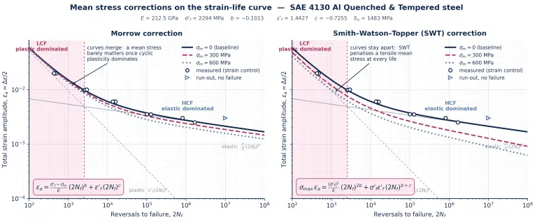
The difference is not cosmetic. At $\sigma_m$ = 300 MPa, Morrow removes about 2% of life at 10² reversals but 73% at 10⁷; SWT removes 25% and 97% at the same two points. Deep in LCF a correction is close to a rounding error — as it should be, since the mean stress has already relaxed.

No single correction wins everywhere, and the ranking can reverse: for this steel, where σ’f sits well above the tensile strength, SWT is more conservative at long lives while Morrow becomes more conservative at short lives and high mean stress. Choose on the sign of your mean stress, validate against test data at the relevant life, and check your stabilized loop first — if the mean stress has already relaxed, the correction is doing almost nothing and should not drive your conclusions.
FEA Workflow for Low Cycle Fatigue Analysis
FEA-based LCF assessment needs three things linear analysis does not: an elastic-plastic material model with kinematic hardening, cyclic (not monotonic) stress-strain data, and a stabilized hysteresis loop extracted at the critical location. The chain is a nonlinear static or transient solve for the plastic strain distribution, then strain-life post-processing.
Material Model Selection and Cyclic Plasticity
Isotropic hardening cannot represent reversed plastic flow — it misses the Bauschinger effect entirely and gives the wrong loop. Kinematic hardening is mandatory. Armstrong-Frederick works for simple cases; the Chaboche model, with several superposed backstress terms, represents cyclic stress-strain response far better for most engineering metals and is the usual production choice.
Calibrate against cyclic stress-strain curves, not monotonic tensile data — a material that softens cyclically has a stabilized loop nothing like its monotonic curve, and calibrating on the wrong data can put your strain range out by a large factor. The stabilized-cycle assumption holds for constant amplitude loading; variable amplitude histories may need cycle-by-cycle simulation.
Mesh and Element Considerations for Strain Accuracy
Plastic strain gradients at stress concentrations are steeper than elastic stress gradients, so LCF analysis demands more mesh refinement than a linear elastic check would. Aim for at least 3–4 elements through the plastic zone at critical locations.
Element formulation matters too. Reduced-integration elements can hourglass under large plastic strain — use enhanced hourglass control or full integration in the critical region. Tighten convergence beyond defaults as well; residual force tolerances of 0.1% or better are advisable if you intend to trust the extracted plastic strain.
Post-Processing and Life Prediction
- Define geometry & boundary conditions
- Define nonlinear material model
- Run the nonlinear analysis with an appropriate cyclic plasticity model
- Cycle until the hysteresis loop at the critical location stabilizes
- Extract the plastic strain range ($\Delta\varepsilon_p$) from the stabilized loop. Check the mean stress in that loop and apply a correction only if it has not relaxed
- Apply the Coffin-Manson or total strain-life relation with validated material constants
- Solve for cycles to failure ($N_f$)

To learn more about high cycle fatigue and fatigue testing procedure, please read: High Cycle Fatigue and Fatigue testing.
Frequently Asked Questions (FAQ)
What is meant by low cycle fatigue?
Low cycle fatigue is failure under high-amplitude cyclic loading where the material yields and deforms plastically on every cycle. Unlike high cycle fatigue, which stays macroscopically elastic, LCF accumulates damage through reversed plastic flow and typically fails between roughly 100 and 10,000 cycles.
How many cycles is considered low cycle fatigue?
Usually under 10,000 cycles, with some references drawing the line nearer 10³. But cycle count is not the definition — the defining feature is macroscopic plastic deformation in each cycle. The material-specific boundary is the transition life 2Nt, where the elastic and plastic strain components are equal.
What is the difference between high cycle and low cycle fatigue?
High cycle fatigue stays below yield, is governed by stress amplitude, takes 10⁵–10⁷ cycles, and is handled with S-N methods. Low cycle fatigue involves plastic deformation each cycle, is governed by strain amplitude, and needs strain-life analysis via Coffin-Manson — and its loading is frequently strain-imposed rather than stress-imposed.
How to calculate low cycle fatigue life?
Use the Coffin-Manson relation, $\frac{\Delta\varepsilon}{2} = \varepsilon’_f (2N_f)^c \tag{2}$ .Take the plastic strain range from a stabilized hysteresis loop in your FEA results, obtain ε’f and c from strain-controlled testing or a validated database, apply a mean stress correction if the mean stress has not relaxed, and solve for Nf.
What is a low cycle fatigue life example?
Gas turbine disk cracking driven by startup and shutdown cycles. Thermal gradients and centrifugal load together push the blade attachment slots past yield every operational cycle, and because the expansion mismatch imposes strain rather than stress, the problem is strain-life by nature.
Does mean stress matter in low cycle fatigue?
Less than you might expect at high strain amplitudes. Cyclic plasticity relaxes mean stress toward zero through plastic shake-down, so corrections do little deep in the LCF regime. They matter in the transition band and at longer lives, where the elastic component dominates and relaxation is incomplete.
References
- Schijve, J., “Fatigue of Structures and Materials”, 2009.
- Yin, F. and Fatemi, A., SAE 4130 Al Quenched & Tempered Steel, Iteration #29: Microstructural Data, Monotonic and Fatigue Test Results. Department of Mechanical, Industrial and Manufacturing Engineering, University of Toledo, Toledo, OH. Prepared for the AISI Bar Steel Applications Group, American Iron and Steel Institute, Southfield, MI, June 2000. Constants from Table 2; test data from Table A.2. Available: https://fde.uwaterloo.ca/Fde/Materials/SMDIdbase/Steel/FatigueReports/Iter_029.pdf
- Morrow, J., “Fatigue Properties of Metals,” Section 3.2, in Fatigue Design Handbook, Graham, J.F. (ed.), Publication No. AE-4, Society of Automotive Engineers, Warrendale, PA, 1968.
- Smith, K.N., Watson, P. and Topper, T.H., “A Stress-Strain Function for the Fatigue of Metals,” Journal of Materials (ASTM), Vol. 5, No. 4, December 1970, pp. 767–778.
- Manson, S.S. and Hirschberg, M.H., “Fatigue Behavior in Strain Cycling in the Low- and Intermediate-Cycle Range,” in Fatigue: An Interdisciplinary Approach, Burke, J.J., Reed, N.L. and Weiss, V. (eds.), Syracuse University Press, 1964, p. 133.
- ASTM E606/E606M, Standard Test Method for Strain-Controlled Fatigue Testing, ASTM International, West Conshohocken, PA.

I am a mechanical engineer in the fields of thermal energy storage, fluid mechanics and heat transfer. I have obtained my PhD from KTH Royal Institute of Technology in designing robust and compact additively manufactured prototypes. During my PhD, I worked on CFD modeling and optimization of innovative heat exchanger designs and conducted experiments of the manufactured prototypes in laboratory environments.
In June 2019, I managed to secure the funding for continuation of my PhD by receiving a grant of 3.7 MSEK from the Swedish Energy Agency on development of 3D-prineted air-PCM heat exchangers.
I am a mechanical engineer in the fields of thermal energy storage, fluid mechanics and heat transfer. I have obtained my PhD from KTH Royal Institute of Technology in designing robust and compact additively manufactured prototypes. During my PhD, I worked on CFD modeling and optimization of innovative heat exchanger designs and conducted experiments of the manufactured prototypes in laboratory environments.
In June 2019, I managed to secure the funding for continuation of my PhD by receiving a grant of 3.7 MSEK from the Swedish Energy Agency on development of 3D-prineted air-PCM heat exchangers.