Understanding Stress-Strain Behavior in Materials: A Comprehensive Guide for FEA and CAE
Learn how stress-strain relationships affect material performance in FEA simulations and CAE modeling. This guide covers uniaxial stress-strain curves, engineering vs. true stress, and strain hardening models essential for accurate finite element analysis.
Understanding stress-strain behavior is fundamental in mechanical engineering, material science, and structural analysis. Whether designing aerospace components, automotive structures, or load-bearing materials, engineers must comprehend how materials respond under loading conditions. This comprehensive guide covers uniaxial stress-strain relationships, engineering vs. true stress, plastic deformation, strain hardening models, and their importance in Finite Element Analysis (FEA) simulations.
Engineering Stress-Strain Relationships
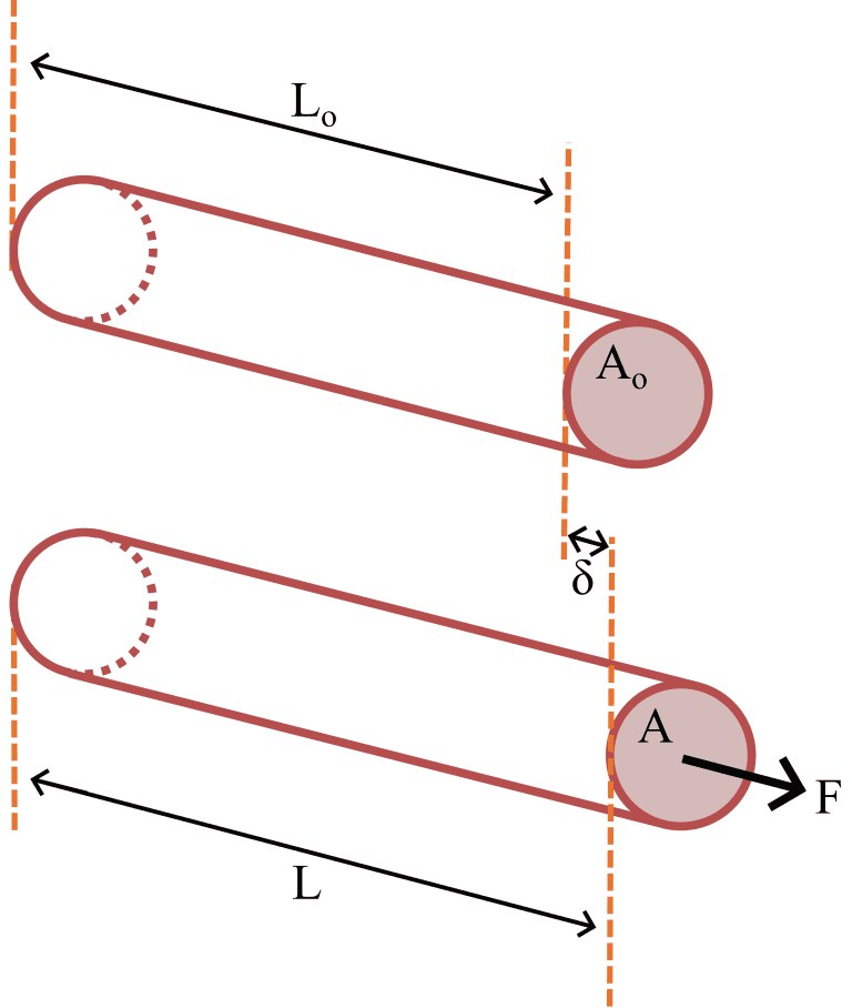
Normal stress refers to the force applied in axial direction to a component, such as a rod, divided by its cross-sectional area, as shown below. When the initial area of the component is used in the definition the obtained stress is referred to as nominal stress.
\[\sigma_{nominal} = \frac{F}{A_0} \tag{1}\]
When a load is applied, the rod undergoes deformation, resulting in an elongation as shown in Figure 1. Normal uniaxial strain is defined as the ratio of the change in the rod’s length to its original length under the applied normal load.
\[\varepsilon_{nominal} = \frac{\delta}{L_0} \tag{2}\]
The nominal stress and strain are referred to as engineering stress and engineering strain in technical literature and FEA documentation.
As the force increases, this uniaxial elongation grows. By plotting stress against strain under increasing load, a stress-strain curve is generated. Materials can generally be classified into two categories—ductile and brittle—based on their behavior observed in a stress-strain curve, which is critical information for FEA simulation setup.
Ductile material
Stress remains proportional to strain up to the yield limit. This region is known as the elastic zone, where the material returns to its original shape when the load is removed. In this zone, stress and strain are linearly related through the modulus of elasticity. Beyond the yield limit, the material enters the plastic region, where relatively large deformations occur with small increases in load. In this region, the material undergoes permanent deformation, no longer returning to its original shape even after the load is removed.
The engineering stress-strain diagram of low carbon steel is shown in Figure 2-a. In materials like low-carbon steel, the yield limit is well-defined and exhibits distinct characteristics. The upper yield point represents the transient maximum load reached just before the material begins to yield. This is followed by the lower yield point, which corresponds to the load required to sustain yielding as the material undergoes plastic deformation. The lower yield point is often used as the reference yield value.
Beyond the yield point, the material undergoes strain hardening as it approaches the ultimate stress, the maximum engineering stress the material can withstand. If the load is increased beyond this ultimate stress, the cross-sectional area of the component begins to decrease significantly in a localized region, a phenomenon known as necking. This stage marks the onset of instability, leading eventually to the material’s fracture.
In certain materials, such as aluminum as shown in Figure 2-b, the yield point is not clearly defined. As the material transitions into the plastic region, the stress increases non-linearly until it reaches the ultimate stress. To determine the yield point in such cases, the offset method is commonly used. This involves drawing a line parallel to the initial linear portion of the stress-strain curve, intersecting the strain axis at a specified offset value. An offset of 0.2% (or 0.002 strain) is widely accepted as a standard for defining the yield point in materials with indistinct yielding behavior.

Brittle material
A brittle material, shown in Figure 3, fractures with little to no significant deformation, exhibiting minimal plasticity before failure. In these materials, the stress at fracture is essentially equal to the ultimate stress, as they lack the capacity to undergo substantial deformation prior to breaking.

True stress-strain VS engineering stress-strain
In calculation of engineering stress it is assumed that the cross-sectional area of the component remains constant. Though in reality the material under an increasing load experiences a continuous reduction in the cross-section area. True stress is defined as the applied load divided by the actual cross-sectional area of the material at a given point during deformation.
True strain is calculated by dividing the material’s length into infinitesimally small segments and integrating the incremental local strains to determine the total strain. True strain can be calculated as a function of the engineering strain as shown below:
\[
\varepsilon_i = \frac{dL_i}{L_i} \tag{3}
\]
\[
\varepsilon_{\mathrm{true}}
= \int_{L_0}^{L} \frac{dL}{L}
= \ln\!\Bigl(\frac{L}{L_0}\Bigr)
\]
Taking the final length as:
\[
L = L_0 + \Delta L
\;\Longrightarrow\;
\varepsilon_{\mathrm{true}}
= \ln\!\Bigl(\frac{L_0 + \Delta L}{L_0}\Bigr)
= \ln\!\bigl(1 + \varepsilon_{\mathrm{nom}}\bigr)
\tag{4}
\]
By having the definition of stress the engineering and true stresses could be correlated as below:
\[
\frac{\sigma_{\mathrm{true}}}{\sigma_{\mathrm{nom}}}
= \frac{A_0}{A_{\mathrm{true}}}
\tag{5}
\]
If it would be assumed that the volume of the material remains constant under loading, true stress can be calculated as below:
\[
A_0\,L_0 = A_{\mathrm{true}}\,L
\;\Longrightarrow\;
\frac{A_0}{A_{\mathrm{true}}}
= \frac{L}{L_0}
= \frac{L_0 + \Delta L}{L_0}
= 1 + \varepsilon_{\mathrm{nom}}
\tag{6}
\]
\[
\sigma_{\mathrm{true}}
= \sigma_{\mathrm{nom}}\,(1 + \varepsilon_{\mathrm{nom}})
\tag{7}
\]
The true stress-strain diagram of a ductile material which takes into account continuous changes of the cross-sectional area is schematically illustrated in Figure 4.

When performing a finite element analysis the output is given always as true stress and strain. However, to perform such an analysis beyond the elastic zone the true strain-stress needs to be given to the software as input.
Plastic deformation and strain hardening
After yield is reached further loading causes more deformation and plastic strain. The total strain can be expressed as the sum of two components: plastic strain and elastic strain.
\[
\varepsilon_{\mathrm{total}}
= \varepsilon_{\mathrm{elastic}}
+ \varepsilon_{\mathrm{plastic}}
\tag{8}
\]
The elastic component is not constant but depends on the current stress, defined by the stress at deformation by the modulus of elasticity:
\[
\varepsilon_{\mathrm{elastic}}
= \frac{\sigma}{E}
\tag{9}
\]
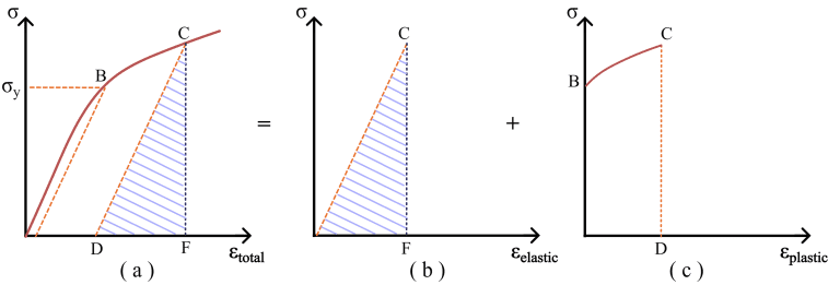
At an arbitrary point of C if the load is removed, the stress returns to zero value in a path parallel to the modulus of elasticity (CD). If the component would be loaded again the stress increases linearly to a higher value of yield (CD) and then continues beyond in a non-linear way. The increase of yield stress in the plastic region is known as strain hardening. Strain hardening does not imply that the material becomes inherently stronger. Here, within the structure during loading/unloading, a system of residual tensile and compressive strains develops, balancing each other out. Upon reloading, the yield limit increases slightly. With repeated cycles of loading and unloading, the yield stress continues to rise incrementally. However, this does not make the material harder; instead, it causes the initially ductile material to exhibit increasingly brittle behavior. It should be noted while during the process yield stress increases the ultimate stress remains the same.
Types of strain hardening:
- Perfectly plastic: in perfectly plastic hardening no unloading occurs. The stress increases with a slope as load increases and rather large plastic deformations happen at little increase in the applied load until the material reaches its ultimate tensile stress.
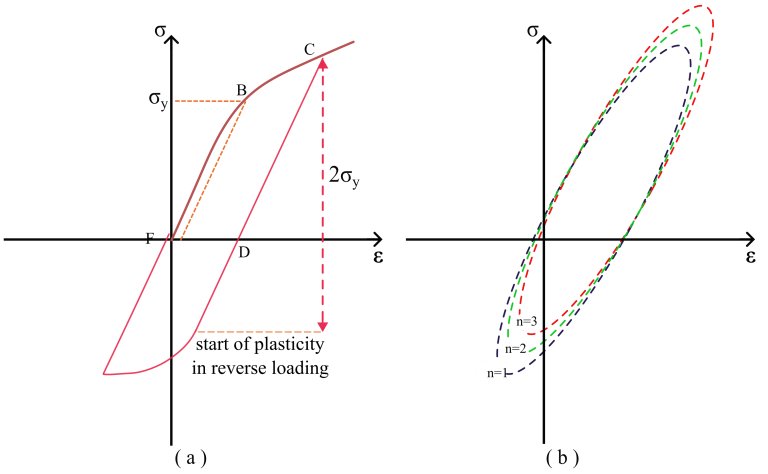
- Isotropic hardening: In isotropic hardening, shown in Figure 6, the material’s yield stress increases uniformly in all directions, maintaining isotropic behavior. This implies that during reverse loading, the stress required to initiate plastic deformation is equal in magnitude but opposite in direction to the initial loading stress. The stress-strain relationship during loading and unloading resembles an elliptical shape. In another word, the hardening occurs to be symmetric and in all directions. This behavior can be observed in materials subjected to loading conditions, such as tubes under combined tension-pressure or tension-torsion loads.

- Kinematic hardening: in kinematic hardening, shown in Figure 7, when reverse load starts after the material entered the plastic zone under a tension force, it typically requires a compressive stress equal to twice the yield stress to undergo plastic deformation in reverse loading. Upon loading again the material experiences a higher yield stress. The yield surface in stress space shifts to a new position without changing its size or shape. This shift represents the directional nature of hardening, primarily influenced by the initial loading path. Unlike isotropic hardening, where hardening occurs uniformly in all directions, kinematic hardening exhibits a strong directional bias along the loading direction.
- Combined hardening: In practice, material hardening behavior often falls somewhere between purely isotropic and purely kinematic. In such cases upon reverse loading it is not completely clear at what stress the plastic deformation begins. This is referred to as the Bauschinger effect. In overall, in this case the hardening is not symmetric in loading and reverse loading directions.
True stress-strain curve as input for FE analysis
To perform accurate Finite Element (FE) analysis, the material’s true stress-strain curve is required. However, test data typically provide engineering stress and strain, derived from measured force and changes length during test. Using the equations above, the true stress and strain can be obtained based on measured engineering stress and strain.
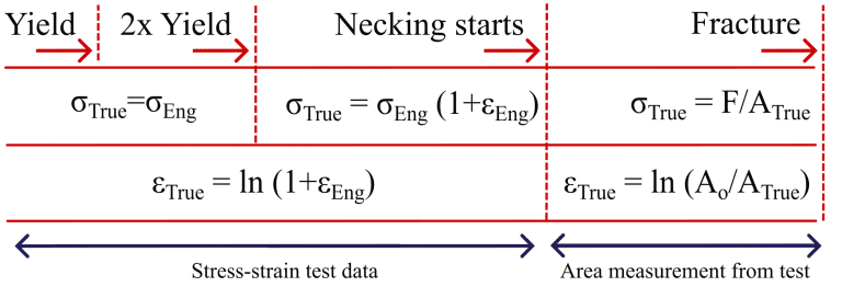
Up to the ultimate stress the true strain can be calculated using the obtained correlation of \(\displaystyle \varepsilon_{\mathrm{true}} = \ln\bigl(1 + \varepsilon_{\mathrm{nom}}\bigr)\). However, since the elastic deformation is associated with volume change the correlation \(\displaystyle \sigma_{\mathrm{true}} = \sigma_{\mathrm{nom}}\,(1 + \varepsilon_{\mathrm{nom}})\) cannot be used. In practice, due to insignificant differences between the true stress and engineering stress up to twice the yield strain, the true stress can be considered the same engineering stress.
It is recommended to avoid taking the assumption of constant volume in cases with small plastic strain. As the material undergoes significant plastic deformation beyond twice the yield strain, the condition of constant volume is fulfilled and true stress can be calculated based on engineering stress.
As during the plastic deformation necking starts, the obtained correlations between the true stress-strain and engineering strain-strain are no longer valid. At this point to calculate the true stress the continuously changing cross-sectional are needs to be measured. In this region the true stress and strain could be calculated using the following equations:
\[
\sigma_{\mathrm{true}} \;=\; \frac{F}{A_{\mathrm{true}}}
\tag{10}
\]
\[
\varepsilon_{\mathrm{true}} \;=\; \ln\!\Bigl(\frac{A_{0}}{A_{\mathrm{true}}}\Bigr)
\tag{11}
\]
The table below summarizes the suitable correlations to extract true stress-strain data.

Amir Abdi holds a PhD in Mechanical Engineering from KTH Royal Institute of Technology, specializing in heat transfer improvement in latent thermal energy storage. He has two years of experience as a CAE Engineer at Scania’s Industrial Operations Asia division and currently works as a Climate Engineer at Envirotainer Engineering AB. Amir’s professional interests include structural mechanics, finite element analysis (FEA), computational fluid dynamics (CFD), and advanced heat transfer. His background combines hands-on engineering experience with in-depth research, enabling him to tackle complex industrial and technological challenges in energy and climate control systems.
Amir Abdi holds a PhD in Mechanical Engineering from KTH Royal Institute of Technology, specializing in heat transfer improvement in latent thermal energy storage. He has two years of experience as a CAE Engineer at Scania’s Industrial Operations Asia division and currently works as a Climate Engineer at Envirotainer Engineering AB. Amir’s professional interests include structural mechanics, finite element analysis (FEA), computational fluid dynamics (CFD), and advanced heat transfer. His background combines hands-on engineering experience with in-depth research, enabling him to tackle complex industrial and technological challenges in energy and climate control systems.