Key Takeaways
Low Cycle Fatigue (LCF) occurs below 10,000 cycles with significant plastic strain; High Cycle Fatigue (HCF) occurs above 10,000 cycles with elastic-dominated response.
Use strain-life (ε-N) methods for LCF; stress-life (S-N) methods for HCF.
Calculate plastic-to-elastic strain ratio to confirm regime classification.
Transition regime (10³–10⁴ cycles) requires combined Coffin-Manson-Basquin approaches
- Fractographic evidence validates analysis assumptions—smooth surfaces indicate HCF, rough surfaces with plastic deformation indicate LCF.
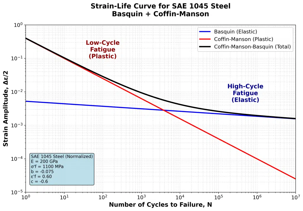
Table of Contents
Introduction
Misclassifying the fatigue regime ranks among the most consequential errors in FEA—components fail prematurely or get massively over-designed when stress-life methods are applied to plastic strain conditions, or strain-life approaches to elastic-dominated loading. Understanding high cycle fatigue and low cycle fatigue fundamentally changes how fatigue life prediction, material characterization, and simulation workflows are approached. This guide covers the mechanisms driving fatigue damage, establishes clear cycle count thresholds, compares material testing requirements, and outlines distinct FEA strategies for each regime—enabling confident methodology selection for turbine blades, pressure vessels, automotive components, and any cyclically loaded structure.
Fundamental Mechanisms: How HCF and LCF Damage Differs
High cycle fatigue occurs when cyclic stress remains below yield strength, causing damage through elastic deformation over hundreds of thousands cycles. Low cycle fatigue involves plastic deformation at stress levels exceeding yield, causing failure in fewer than 10,000 cycles through strain-controlled mechanisms.
Elastic vs. Plastic Strain Dominance
The defining characteristic separating these regimes lies in the stress-strain response during cycling. Understanding the difference between high cycle fatigue and low cycle fatigue begins with recognizing which strain component dominates the material response.
The Coffin-Manson equation captures how plastic strain amplitude relates to fatigue life when significant plasticity occurs during each cycle, making it the governing relationship for LCF analysis. Basquin’s equation, in contrast, applies to the elastic-dominated regime where stress amplitudes remain below yield.
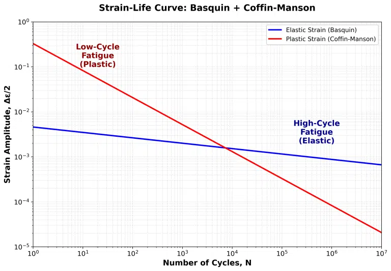
When plotting strain-life data on log-log coordinates, Basquin’s equation governs the elastic strain component while Coffin-Manson governs the plastic strain component. The combined total strain curve—often called Morrow’s relationship—represents their sum. Where these two curves intersect defines the transition life (2Nt), marking the boundary where material behavior shifts from plastic-dominated to elastic-dominated failure mechanisms. This transition life concept is critical—it tells you where one mechanism begins to dominate over the other for a specific material.
💡 Pro Tip: When evaluating a new component, calculate the ratio of plastic to elastic strain amplitude at your maximum loading condition. If plastic strain exceeds elastic strain, you’re firmly in LCF territory regardless of expected cycle count.
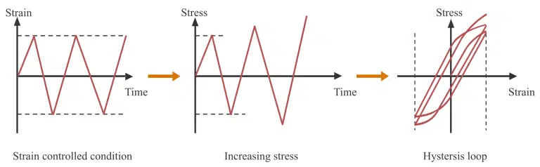
For cyclic loading producing plastic strains, the material response forms a hysteresis loop rather than following a linear elastic path. The area within this loop represents energy dissipated per cycle—energy that accumulates as fatigue damage. In HCF, these loops are narrow (nearly elastic), while LCF produces wide hysteresis loops indicating significant plastic work per cycle. This hysteresis behavior directly influences how engineers approach fatigue strength assessment for each regime.
Crack Initiation and Propagation Differences
In high cycle fatigue, crack initiation dominates total fatigue life. Surface defects, inclusions, and stress concentrations serve as nucleation sites where microscopic cracks form after millions of elastic stress cycles. The propagation phase is relatively short compared to initiation. Surface conditions become extremely important—surface hardening treatments and cold rolling introduce beneficial compressive residual stresses that improve fatigue resistance.
Low cycle fatigue reverses this relationship. The significant plastic deformation per cycle accelerates crack initiation, making the propagation phase a more substantial portion of total life. This has direct implications for inspection intervals and damage tolerance approaches—LCF components may require more frequent inspection once cracks are detected because propagation proceeds more rapidly relative to total life.
Cycle Count Thresholds: Defining the HCF-LCF Boundary
Low cycle fatigue typically encompasses failures occurring below 10,000 cycles (10⁴), while high cycle fatigue describes failures between 10,000 and 10 million cycles (10⁴–10⁷). The transition zone between 1,000–10,000 cycles requires careful analysis of strain components to determine the dominant mechanism.
Industry-Specific Classification Standards
The boundary separating high cycle fatigue and low cycle fatigue lacks universal agreement, with various sources placing the transition anywhere between 10³ and 10⁵ cycles. However, different industries adopt different thresholds based on safety factors and loading characteristics:
| Industry | LCF Threshold | HCF Range | Rationale |
|---|---|---|---|
| Aerospace | Often 10³ cycles | 10³–10⁷ | Conservative approach for safety-critical rotating components |
| Power Generation | 10⁴ cycles | 10⁴–10⁷ | Standard threshold for turbine and boiler components |
| Automotive | 10⁴ cycles | 10⁴–10⁶ | Balance between durability and weight optimization |
| Pressure Equipment | 10⁴ cycles | 10⁴–10⁶ | ASME code-based classification |
The Transition Regime Challenge
The 10³–10⁴ cycle range presents a genuine analytical challenge where both elastic and plastic strains contribute significantly to fatigue damage. Material behavior in this regime typically shifts around 10,000 cycles, making this boundary region particularly important for accurate fatigue life prediction.
Within the HCF regime, materials exhibit mixed elastic-plastic behavior rather than purely elastic response. This necessitates combining both Basquin’s stress-based approach and Coffin-Manson’s strain-based approach to accurately characterize the complete S-N curve across the full range of cycles. For transition regime analysis, combined approaches like Morrow or Smith-Watson-Topper (SWT) provide more accurate predictions by accounting for both strain components.
⚠️ Common Mistake: Defaulting to HCF methods for components in the transition regime because “it’s simpler.” This approach often yields non-conservative life predictions when plastic strain contributions are significant.
Material Characterization: Testing and Data Requirements
High cycle fatigue testing uses stress-controlled fatigue tests generating S-N curves, while LCF requires strain-controlled testing producing ε-N curves. Material data must match the dominant deformation mechanism—using S-N data for LCF analysis introduces significant non-conservative error that no amount of safety factor can reliably compensate.
S-N Curves for High Cycle Fatigue Analysis
In the HCF regime, engineers typically characterize fatigue behavior using Basquin’s power-law equation, which establishes a linear relationship between stress amplitude and cycles to failure on a log-log plot.
The stress-life approach requires understanding several key concepts:
- Endurance limit: For certain materials—particularly ferrous alloys like carbon steels—the S-N curve levels off at a threshold stress below which the material can theoretically survive unlimited cycles without fatigue failure. For mild steels, this limit typically falls between 45-50% of ultimate tensile strength, while medium carbon steels may reach 55% of UTS.
- Mean stress corrections: Mean stresses significantly affect HCF behavior. Available correction methods include Soderberg, Goodman, Gerber, Morrow, and Smith-Watson-Topper approaches. Selecting the appropriate correction method significantly impacts fatigue life calculations.
Strain-Life Curves for Low Cycle Fatigue Analysis
LCF analysis relies on the Coffin-Manson relationship, developed independently through the research of L.F. Coffin and S.S. Manson in the early 1950s. Manson’s contribution stemmed from extensive uniaxial testing that revealed the empirical correlation between plastic strain range and fatigue life.
The combined Coffin-Manson-Basquin equation captures total strain amplitude:
$$\frac{\Delta\varepsilon}{2} = \frac{\sigma’ f}{E}(2N)^b + \varepsilon’ f (2N)^c \tag{1}$$
Where:
- $\sigma’ f$= fatigue strength coefficient
- $b$ = fatigue strength exponent (typically -0.12 to -0.05)
- $\varepsilon’ f$= fatigue ductility coefficient
- $c$ = fatigue ductility exponent (typically -0.5 to -0.7)
The fatigue ductility exponent c generally falls between -0.5 and -0.7 for metallic materials under time-independent loading conditions. Materials with higher ductility tend toward values near -0.6, while higher-strength materials with less ductility often exhibit values closer to -0.5. These material constants are essential for accurate strain-life fatigue analysis.
FEA Implementation: Simulation Workflow Differences
High cycle fatigue FEA uses linear elastic stress results with stress-life algorithms, while low cycle fatigue requires elastic-plastic material models capturing cyclic plasticity. Selecting the wrong approach invalidates fatigue life predictions regardless of mesh quality or solver accuracy—this is a methodology error, not a discretization error.
HCF Workflow: Stress-Based Analysis Setup
The HCF workflow leverages linear elastic FE solutions, making it computationally efficient for fatigue analysis:
- Linear elastic FE solution: Standard static or modal analysis provides stress distribution
- Stress extraction: Nodal averaging typically preferred; elemental results for discontinuity regions
- Multiaxial stress handling: Critical plane methods or equivalent stress approaches (von Mises, signed von Mises, maximum principal)
- Cycle counting: Rainflow counting for variable amplitude loading histories
- Damage accumulation: Palmgren-Miner linear damage rule: $ D = \Sigma\frac{n_i}{N_i} $
📋 Quick Reference: For HCF analysis, verify that maximum stress amplitude remains below 80% of yield strength. Above this threshold, localized plasticity may invalidate the linear elastic assumption.
LCF Workflow: Strain-Based Analysis Requirements
Low cycle fatigue (LCF) analysis can be performed using two distinct workflows. Approach 1 employs elastic finite element analysis combined with notch correction methods (Neuber or ESED) to estimate local plastic strains—a fast, practical method widely used in industry.

Approach 2 uses nonlinear finite element analysis with advanced material models (Chaboche or Armstrong-Frederick) to directly capture cyclic plasticity behavior, extracting strains from the stabilized hysteresis loop for more accurate predictions at the cost of increased computational complexity. Both approaches ultimately apply the Coffin-Manson-Basquin strain-life equation to predict component fatigue life. The flowcharts below detail each methodology step-by-step, including their respective advantages and limitations.

Software Considerations and Common Pitfalls
Commercial fatigue solvers (fe-safe, nCode DesignLife, FEMFAT) handle both regimes but require correct setup:
- Material library limitations: Verify that strain-life parameters exist for your material; S-N data is more commonly available
- Mesh sensitivity: LCF results are more mesh-sensitive near stress concentrations due to plastic strain gradients
- Computational cost: Elastic-plastic cycling for LCF can require 10-100x more computation time than linear HCF analysis
⚠️ Common Mistake: Running elastic-plastic FEA for a single load cycle and extracting strains. LCF analysis requires cycling to stabilization—typically 10-50 cycles depending on material hardening behavior.
Failure Characteristics and Fractography
HCF failures exhibit smooth, fine-textured fracture surfaces with distinct beach marks from gradual crack growth. LCF failures show rougher surfaces with visible striations, minimal crack propagation zone, and evidence of gross plastic deformation near the origin. Understanding these signatures enables validation of your analysis assumptions.
Visual Indicators on Fracture Surfaces
Fractographic examination reveals distinct features for each regime:
High Cycle Fatigue Indicators:
- Fine, smooth fracture surface texture
- Distinct beach marks (arrest lines) showing incremental crack growth
- Small final fracture zone relative to total fracture area
- Crack origin typically at surface defect or stress concentration
- Minimal evidence of gross plastic deformation
Low Cycle Fatigue Indicators:
- Rougher, more textured fracture surface
- Coarse striations visible under magnification
- Larger final fracture zone (rapid propagation phase)
- Evidence of plastic deformation near crack origin
- Multiple initiation sites possible under severe loading
Correlating Failure Evidence with FEA Predictions
When physical evidence contradicts your analysis approach, the fractography wins. I’ve encountered cases where HCF analysis predicted adequate life, but fractographic examination revealed LCF characteristics—indicating the loading was more severe than assumed or local plasticity occurred at stress concentrations.
Document the correlation between predicted and observed failure characteristics in your investigation reports. This validation step builds confidence in your methodology for future analyses of similar components.
Practical Applications: Industry Case Examples
Fatigue analysis in real-world applications often involves combined high cycle fatigue (HCF) and low cycle fatigue (LCF) loading scenarios. Understanding how these mechanisms interact is crucial for accurate life prediction in critical components. Two primary industrial applications demonstrate the complexity of combined fatigue loading: rotating machinery (turbine blades) and pressure equipment (vessels and piping systems).
| Application | LCF Contribution | HCF Contribution | Key Considerations |
|---|---|---|---|
| Rotating Machinery (Gas Turbine Blades) |
|
|
|
| Pressure Equipment (Vessels & Piping) |
|
|
|
Summary
The distinction between high cycle fatigue and low cycle fatigue represents one of the most critical decisions in structural durability analysis. Throughout this guide, we’ve established that HCF occurs when cyclic stresses remain below yield strength, producing elastic deformation over millions of cycles, while LCF involves significant plastic strain causing failure within thousands of cycles. This fundamental difference in deformation mechanism dictates every aspect of your analysis approach.
Material characterization requirements differ substantially between regimes. HCF analysis relies on stress-controlled S-N curves with appropriate mean stress corrections, while LCF demands strain-controlled ε-N curves characterized by Coffin-Manson parameters. Using mismatched material data introduces errors that safety factors cannot reliably address—the methodology must match the physics.
FEA implementation strategies diverge based on regime classification. Linear elastic solutions with stress-life algorithms provide computationally efficient HCF analysis, while LCF requires nonlinear elastic-plastic material models or validated notch correction methods. The transition regime between 10³–10⁴ cycles demands combined approaches accounting for both elastic and plastic strain contributions.
Frequently Asked Questions (FAQ)
How many cycles is considered low cycle fatigue?
Low cycle fatigue encompasses failures below 10,000 cycles (10⁴), with some industries using 1,000 cycles as threshold. The defining characteristic is significant plastic strain per cycle rather than strict cycle count—if plastic deformation dominates, LCF methodology applies.
What is low cycle fatigue?
Low cycle fatigue is characterized by two defining features: measurable plastic deformation occurring during each loading cycle, and a limited number of cycles before failure occurs. This strain-controlled process leads to crack initiation and failure within relatively few cycles, requiring strain-life analysis methods.
What is an example of high cycle fatigue?
Common HCF applications include rotating machinery components such as shafts, gears, and turbine blades operating at steady state; aircraft wing structures subjected to repeated aerodynamic loading; automotive springs and connecting rods; and bridge structural members experiencing traffic-induced vibrations. These components experience millions of elastic stress cycles throughout their service life.
What is the difference between HCF and LCF failure?
HCF failure results from millions of low-amplitude elastic stress cycles, producing smooth fracture surfaces with gradual crack growth. LCF failure occurs within thousands of high-amplitude cycles involving plastic strain, creating rougher surfaces with gross deformation evidence.
What is the difference between high cycle fatigue and low cycle fatigue in FEA?
In FEA, high cycle fatigue analysis uses linear elastic stress results with S-N curves, while low cycle fatigue requires elastic-plastic material models with ε-N curves. HCF simulations run faster; LCF demands computationally expensive nonlinear cycling for accurate results.
Can a component experience both high cycle and low cycle fatigue?
Yes, many components experience combined HCF-LCF loading—turbine blades undergo LCF from thermal startup cycles and HCF from vibratory stresses during operation. Analysis requires partitioning damage contributions using interaction models accounting for both mechanisms.
References
- Coffin, L.F. (1954). “A Study of the Effects of Cyclic Thermal Stresses on a Ductile Metal”.
- Manson, S.S. (1953). “Behavior of Materials Under Conditions of Thermal Stress”.
- Basquin, O.H. (1910). “The Exponential Law of Endurance Tests”.
- MMPDS (Metallic Materials Properties Development and Standardization)
- ASME Boiler and Pressure Vessel Code, Section VIII Division 2
- ASTM E606 – Standard Test Method for Strain-Controlled Fatigue Testing
- ASTM E466 – Standard Practice for Conducting Force Controlled Constant Amplitude Axial Fatigue Tests

I am a mechanical engineer in the fields of thermal energy storage, fluid mechanics and heat transfer. I have obtained my PhD from KTH Royal Institute of Technology in designing robust and compact additively manufactured prototypes. During my PhD, I worked on CFD modeling and optimization of innovative heat exchanger designs and conducted experiments of the manufactured prototypes in laboratory environments.
In June 2019, I managed to secure the funding for continuation of my PhD by receiving a grant of 3.7 MSEK from the Swedish Energy Agency on development of 3Dprineted air-PCM heat exchangers.