Fatigue failures causes most mechanical failures in serivce, yet many engineers treat S-N curve interpretation as a black-box without understanding the underlying data, creating risks of catasrophic under-design or costly over-engineering. This article provides practical understanding of S-N curve fundamnetals, construction methods, and application to FEA-driven fatigue analysis. The content helps engineers validate material datasets and troubleshoot unexpected fatigue life predictions, sharpening engineering judgment .
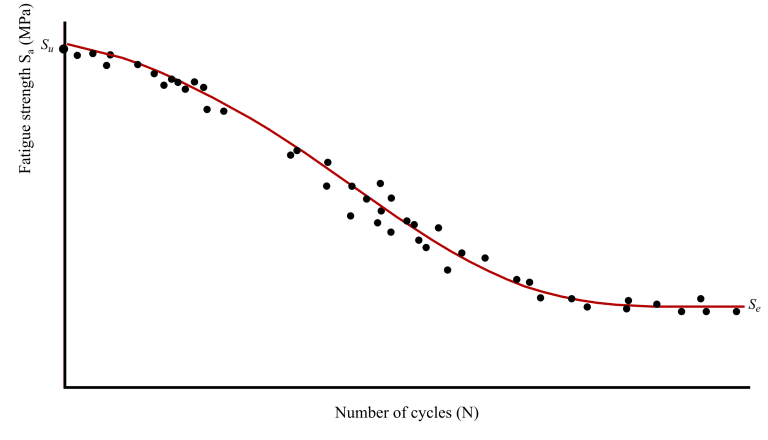
Table of Contents
What Is an S-N Curve and Why It Matters in Fatigue Engineering?
An S-N curve (stress-number curve) is a graphical representation plotting stress amplitude against the number of cycles to failure, enabling engineers to predict fatigue life under cyclic loading conditions.
Also called a Wöhler curve, the S-N curve forms the empirical foundation for high-cycle fatigue analysis in structural and mechanical components. The historical significance of S-N curves cannot be overstated. They were developed by German scientist August Wöhler during investigations following an 1842 train crash in Versailles, France, where a locomotive axle failed under repeated moderate stresses encountered during routine train operations. This pioneering work established that parts subjected to cyclic loading can fail even when peak stresses remain well within static design limits.
The Anatomy of S-N Curve Components
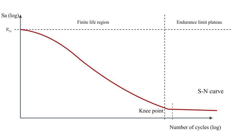
The S-N curve displays stress amplitude (stress range in some references) on the vertical axis against the logarithm of cycles to failure on the horizontal axis. It shows the relationship between the applied load and the fatigue life of a material. The S-N curve is typically separated into different ranges, which differ mainly in their fatigue damage processes.
Three distinct regions characterize most S-N curves:
– Finite life region: The inclined portion where increasing stress amplitude dramatically reduces cycles to failure
– Transition zone (knee point): Where the curve begins to flatten, typically around 10⁶ cycles for steels
– Endurance limit plateau: The horizontal asymptote representing infinite life capability (in practice it follows Haibach-exponent which means the curve is not completely flat).
Figure 1 shows the schematic layout of S-N curve for a common material like steel, desginated by the mentioned regions. Unlike steel, some materials like aluminum show no endurance limit plateua, and the number of cycles increases with decreasing the amplitude stress.
S-N Curves vs. ε-N Curves: Selecting the Right Approach
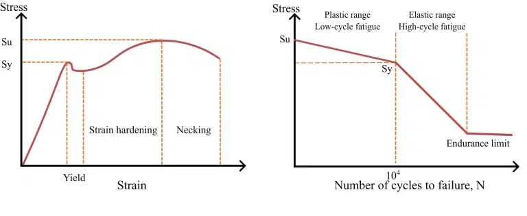
Uniaxial Fatigue Analysis, using S-N (stress-life) and E-N (strain-life) approaches for predicting the life of a structure under cyclical loading may be performed. The stress-life method works well in predicting fatigue life when the stress level in the structure falls mostly in the elastic range. Under such cyclical loading conditions, the structure typically can withstand a large number of loading cycles; this is known as high-cycle fatigue.
When the cyclical strains extend into plastic strain range, the fatigue endurance of the structure typically decreases significantly; this is characterized as low-cycle fatigue. The generally accepted transition point between high-cycle and low-cycle fatigue is around 10,000 loading cycles. Figure 2 shows schematically the engineering stress-strain curve and S-N curve with low- and high-cycle fatigue regions, designated based on the yield and ultimate stresses obtained via the stress-strain cruve. For low-cycle fatigue prediction, the strain-life (E-N) method is applied, with plastic strains being considered as an important factor in the damage calculation.
💡Pro Tip: If your FEA results show localized plasticity at stress concentrations but the bulk of your component remains elastic, consider using strain-life methods locally while applying stress-life globally. Many modern fatigue solvers support this hybrid approach.
How S-N Curves Are Created Through Fatigue Testing
S-N curves are created through controlled fatigue testing where multiple specimens are subjected to constant-amplitude cyclic loading at various stress levels until failure. Each test point represents one stress amplitude and its corresponding cycles to failure, with statistical regression generating the final S-N curve.
Fatigue tests, often involving constant-amplitude cyclic loading, are performed on specimens of the material. The resulting data—stress amplitude and number of cycles to failure for each specimen—is plotted on a log-log scale (log S vs. log N). The slope of the resulting straight line provides the fatigue strength exponent ‘b’, while the intercept gives the fatigue strength coefficient ‘c’.
Conventionally, five different stress levels with three repeats at each level is considered the minimum to determine an S-N curve. However, for critical applications, significantly more testing is required to establish statistical confidence.
Specimen Preparation and Test Standards
Test specimen geometry, surface finish, and preparation consistency directly impact S-N curve data validity. ASTM E466 governs axial fatigue testing procedures, while ASTM E606 covers strain-controlled testing for low-cycle applications.
Statistical Treatment and Scatter Bands
With enough experiments, the S-N curve consists of a series of confidence intervals around the main curve. The curve you see in handbooks is actually a curve fit to a distribution of data points, not a deterministic relationship.
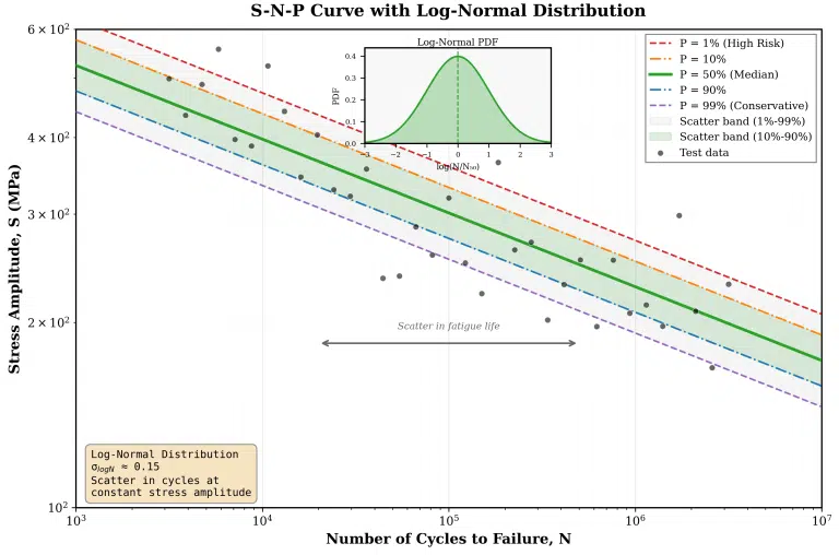
As coupons sampled from a homogeneous frame will display a variation in their number of cycles to failure, the S-N curve should more properly be a Stress-Cycle-Probability (S-N-P) curve to capture the probability of failure after a given number of cycles of a certain stress. Probability distributions that are common in data analysis and in design against fatigue include the log-normal distribution, extreme value distribution, Birnbaum–Saunders distribution, and Weibull distribution.
Waloddi Weibull, a Swedish mathematician, found out at the fatigue rate of failure could not properly described by the log-normal distribution. He carried out experimental studies on structural joint failures under cyclic loading and developed his own distribution, known as Weibull distribution, better representing the fatigue failure probabilities. Figure 3 and 4 show schematic S-N curves with scatter bands for log-nomal and Weibull distributions, with probabilities ranging from 1% to 99%.
Design codes specify which probability curve to use—typically 95% or 99% survival probability for safety-critical applications, versus 50% (mean) for general design. Know which S-N curve your material data represents before applying it.
⚠️ Common Mistake: Using mean (50% survival) S-N data for safety-critical components. Always verify the probability basis of your material curves and apply appropriate knockdown factors for reliability requirements.

The Mathematical Relationship: S-N Curve Formulas and Parameters
The S-N curve formula follows Basquin’s equation:
$$\sigma_a = \sigma’_f (2N_f)^b\tag{1}$$
where $\sigma_a$ is stress amplitude, $\sigma’_f$ is the fatigue strength coefficient, $N_f$ is cycles to failure, and $b$ is the fatigue strength exponent. This power-law relationship appears linear on log-log axes, making it convenient for interpolation and extrapolation within tested ranges.
In 1910, Basquin observed that stress-life (S-N) data could be plotted linearly on a log-log scale. The parameters $\sigma’_f$ and $b$ are fatigue properties of the material that define the S-N curve behavior.
Basquin's Equation and Material Constants
Each parameter in Basquin’s equation carries physical meaning:
– $\sigma’_f$ (fatigue strength coefficient): The fatigue strength coefficient is approximately equal to the true fracture strength at fracture. A good approximation is $\sigma’_f = \sigma_f$ where $\sigma_f$ is ultimate stress.
– b (fatigue strength exponent): The fatigue strength exponent which is the slope of the log-log S-N curve in the high-cycle region, represents the resistane of the material to crack growth in time under cyclic loading.
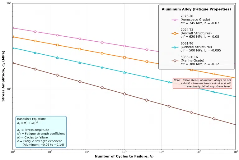
📋 Quick Reference: Typical Basquin exponent ranges for S-N curve characterization: Steels: -0.05 to -0.12 | Aluminum alloys: -0.06 to -0.14 | Titanium alloys: -0.04 to -0.10. Figure 5 and 6 show the S-N curve for some well-known steel and aluminum alloys based on Basquins equation.

Accounting for Mean Stress Effects
Real-world loading rarely produces fully reversed (R = -1) conditions. Mean stress corrections adjust laboratory S-N curve data to actual loading scenarios. For Basquin model, select Soderberg, Goodman, Gerber, Morrow or Smith-Watson-Topper.
The Goodman correction is most commonly used for conservative design, while Gerber provides less conservative predictions that often match test data better for ductile materials. The Goodman-Line is a method used to estimate the influence of the mean stress on the fatigue strength. Your FEA post-processor likely offers multiple options—understand which your industry standards require!
Applying S-N Curves in FEA-Based Fatigue Analysis
In FEA fatigue analysis, S-N curves are applied by extracting cyclic stress results from solved models, and then the curve relationship is used to calculate fatigue life at each node or element. Software interpolates between S-N curve data points to determine the number of cycles to failure for the computed stress state.
Given a load time history and an S-N curve, one can use Miner’s Rule to determine the accumulated damage or fatigue life of a mechanical part. When dealing with variable amplitude loading, the Rainflow counting method transforms irregular load sequences into a series of simplified constant-amplitude cycles suitable for S-N curve analysis.
Material Library Selection and Custom Curve Input
From a given material’s fatigue strength S-N curve, you can derive the Basquin equation constants, or let the program calculate the Basquin constants by specifying the number of data points on the S-N curve to include in the curve-fitting calculations. Most commercial fatigue solver software packages (nCode, FEMFAT) include material libraries, but these generic curves may not match your specific alloy heat treatment, processing, or surface condition.
The book “FKM Analytical Strength Assessment” published by the VDMA (German engineering association) contains many material S-N curves and is widely referenced for European applications.
Interpreting Fatigue Life Contour Results
Damage accumulation follows Miner’s linear damage rule states that failure occurs when cumulative damage D reaches 1.0,
$$D = \Sigma \frac{n_i}{N_i}\tag{2}$$
where $n_i$ is cycles applied at stress level i and $N_i$ is cycles to failure at that stress. While Miner’s rule has known limitations (it ignores sequence effects), it remains the industry standard for most applications. This work flow is breifly explained here.
When a mechanical component experiences repeated loading over time, it accumulates fatigue damage that can eventually lead to failure—even if the stresses never exceed the material’s ultimate strength. To predict how long a part will last, engineers rely on two key pieces of information: the load time history (the record of how stress varies over time during operation) and the S-N curve (a material property that tells us how many cycles at a given stress level the material can withstand before failure). The challenge is that real-world loading is rarely constant—components experience a mix of high, medium, and low stress cycles in irregular patterns. This is where rainflow cycle counting comes in: it’s a method that analyzes the complex load history and breaks it down into individual cycles, each with a specific stress range, that can be counted and categorized.

Once the cycles are extracted and sorted by stress level, Miner’s Rule provides a straightforward way to calculate the total accumulated damage. The rule states that each cycle consumes a fraction of the component’s fatigue life—specifically, if a part experiences n cycles at a stress level where the S-N curve predicts failure at N cycles, then the damage from those cycles is simply n/N. The total damage D is the sum of these fractions across all stress levels. When D reaches 1.0, the part is predicted to fail. For example, if the calculated damage is 0.01, the component can theoretically survive about 100 repetitions of that load history. In practice, different industries use more conservative values for part failure prediction (e.g. D = 0.1-0.3)
The limitation of Miner rule is that the orders and sequences in which the cyclic loads were applied are not considered. However, this simple linear damage accumulation model, while not perfect, provides engineers with a practical tool for estimating fatigue life under variable amplitude loading conditions.
💡 Pro Tip: Fatigue results are highly mesh-sensitive at stress concentrations. Always perform mesh convergence studies on fatigue life predictions, not just peak stress values. A 5% change in stress can translate to 50%+ change in predicted life due to the logarithmic nature of S-N curve relationships.
Critical Factors Affecting S-N Curve Accuracy
S-N curve accuracy depends on modification factors including surface finish ($k_s$), size effect ($k_d$), reliability ($k_r$), and loading type ($k_l$). Raw laboratory data must be adjusted using these factors to reflect actual component conditions, often reducing the endurance limit by 50% or more.
The progression of the S-N curve can be influenced by many factors such as corrosion, temperature, residual stresses, and the presence of notches.
Surface, Size, and Environmental Corrections
Laboratory specimens feature polished surfaces and small cross-sections—conditions rarely matched in production components. The Shigley/Mischke methodology provides systematic correction factors:
- Surface factor $k_s$: Accounts for as-machined, ground, or as-forged surface conditions
- Size factor $k_d$: Larger components have higher probability of containing critical defects
- Reliability factor $k_r$: Adjusts from 50% survival to required reliability level
- Loading factor $k_l$: Corrects for bending vs. axial vs. torsional loading
These factors compound multiplicatively. A component with machined surface, 50mm diameter, and 99% reliability requirement might see its effective endurance limit reduced to 40% of published S-N curve values.
Conclusion
The S-N curve provides the empirical foundation for high-cycle fatigue life prediction, relating stress amplitude directly to cycles to failure through Basquin’s power-law relationship. Understanding this relationship—not just applying it blindly—separates competent fatigue analysis from checkbox engineering.
Raw laboratory S-N curve data requires modification factors for surface finish, size, reliability, and loading type before application to real components. Neglecting these corrections leads to non-conservative designs that may fail in service. FEA-based fatigue workflows depend on appropriate curve selection, proper mean stress correction, and understanding of the underlying test conditions that generated the material data.
Statistical scatter in fatigue data necessitates probability-based design approaches, particularly for safety-critical applications. Know whether your S-N curves represent 50% or 95% survival probability before committing to a design.
Your next step: Audit your current FEA fatigue workflow by verifying that material S-N curves match your component’s surface condition, size, and loading type. Apply appropriate modification factors before your next analysis submission—your designs and your reputation depend on it.
Finally, if you want to know more about fatigue testing, please click on below and read the following blog :
Fatigue Testing: Complete Guide to Professional Services for FEA Validation
Frequently Asked Questions (FAQ)
What is the S-N curve?
The S-N curve is a fatigue characterization plot showing the relationship between applied stress amplitude and the number of loading cycles a material withstands before failure. It enables engineers to predict component fatigue life under cyclic loading and forms the basis for high-cycle fatigue design calculations.
What is the formula for the S-N curve?
The standard S-N curve formula is Basquin’s equation: $\sigma_a = \sigma’_f (2N_f)^b$. Here, $\sigma_a$ represents stress amplitude, $\sigma’_f$ is the fatigue strength coefficient, $N_f$ is the number of cycles to failure, and $b$ is the fatigue strength exponent (typically -0.05 to -0.12 for metals).
How is an S-N curve created?
S-N curves are created through systematic fatigue testing where identical specimens undergo constant-amplitude cyclic loading at different stress levels until failure occurs. Each test generates one data point; statistical regression through multiple points at various stress levels produces the characteristic curve.
How do you use an S-N curve in fatigue analysis?
Engineers use S-N curves by entering the cyclic stress amplitude from their analysis (FEA or hand calculation) and reading the corresponding fatigue life. For variable amplitude loading, damage from each stress level is summed using Miner’s rule until cumulative damage reaches 1.0.
Where can I find S-N curves for specific materials?
S-N curve data sources include material supplier datasheets, MMPDS handbook, ASM Handbooks, FKM guidelines, FEA software material libraries, and published literature. For critical applications, custom testing matching actual component conditions is recommended.
What is the endurance limit on an S-N curve?
The endurance limit is the stress amplitude below which a material theoretically sustains infinite cycles without fatigue failure. It appears as a horizontal asymptote on the S-N curve, typically occurring around 10⁶-10⁷ cycles for ferrous metals. Non-ferrous alloys generally lack a true endurance limit.
References:
Bannantine, J., (2012). Fundamentals of Metal Fatigue Analysis (1 st. ed). Pearson
Haibach, E., (2003). FKM-Guideline, Analytical Strength Assessment of components in mechanical engineering, (5 th. ed)

I am a mechanical engineer in the fields of thermal energy storage, fluid mechanics and heat transfer. I have obtained my PhD from KTH Royal Institute of Technology in designing robust and compact additively manufactured prototypes. During my PhD, I worked on CFD modeling and optimization of innovative heat exchanger designs and conducted experiments of the manufactured prototypes in laboratory environments.
In June 2019, I managed to secure the funding for continuation of my PhD by receiving a grant of 3.7 MSEK from the Swedish Energy Agency on development of 3Dprineted air-PCM heat exchangers.