Yield Criteria under Combined Loading

Learn how yield stress for a specimen under uniaxial loading could be used for a component loading

Accurate prediction of material yielding under complex loading conditions is fundamental to computer-aided engineering (CAE), where virtual prototypes replace physical testing to save cost and time. Yield criteria, such as maximum shear stress theory and distortion energy theory, enable engineers to predict failure in components subjected to combined loads like torsion-pressure combinations or multi-directional forces. These theories provide a mathematical bridge between simplified uniaxial tensile test data and real-world multiaxial stress states. In other words, they allow engineers to use the yield data of a test specimen to predict failure in components under combined loading. This capability forms the cornerstone of reliable finite element analysis (FEA). In this blog, the most well-known theories for ductile and brittle materials are introduced and explained.

Why yield criteria are needed for components subjected to combined loading?

In a uniaxial tensile stress test, as the material enters the plastic region, the normal stress in the direction of the applied force obtained from the test is considered the yield stress. Therefore, under similar conditions, regardless of the actual mechanism that causes the material to yield, it can be said that the material yields when the normal stress reaches the yield stress obtained from the test.

However, when a component is subjected to forces in more than one direction, the yield stress from a uniaxial tensile test cannot be directly used as the yield criterion. In such cases, it is necessary to link the yield mechanism in the component under combined loading to the mechanism that causes yielding in the specimen during a uniaxial test. In this way, a yield criterion for combined loading can be defined based on the data from the uniaxial tensile test.

Yield criteria for ductile materials

The most well-known criteria for ductile materials are maximum shear stress and maximum distortion energy criterion.

Maximum Shearing Stress

It is understood that, in a specimen under uniaxial loading, the mechanism that causes yielding is the slippage of microscopic oblique surfaces within the material, primarily due to shear stress. Thus, it is stated that the material has not yielded if the maximum shear stress in the component under combined loading is below the maximum shear stress observed in the specimen during the uniaxial test.

\[ \left( \tau_{\text{max}} \right)_{\text{component}} < \left( \tau_{\text{max}} \right)_{\text{test specimen}} \tag{1} \]

To obtain the maximum shear stress under uniaxial or biaxial loading, the Mohr’s circle method can be used.

For a three-dimensional element under uniaxial stress, it can be shown that the maximum shear stress at yield is equal to half of the yield stress.

\[\tau_{\text{max}} = \frac{\sigma_Y}{2}\tag{2}\]

Now imagine that an element is subjected to biaxial stress in a plane, where the stress in the third dimension—perpendicular to the plane—is zero. This condition is referred to as plane stress. In the case of plane stress, it can be shown that the maximum shear stress depends on the type of stress, and it can be categorized as follows:

\[
\tau_{\text{max}} = \frac{|\sigma_1|}{2} < \frac{\sigma_Y}{2}\tag{3}
\]

\[
\tau_{\text{max}} = \frac{|\sigma_2|}{2} < \frac{\sigma_Y}{2}\tag{4}
\]

\[
\tau_{\text{max}} = \frac{|\sigma_1 – \sigma_2|}{2} < \frac{\sigma_Y}{2}\tag{5}
\]

A more detailed explanation of how the maximum shear stresses above are obtained using Mohr’s circle is provided here. Plotting the resulting criterion on the principal stress coordinates $\sigma_1$ and $\sigma_2$ forms a hexagon known as the Tresca hexagon, as shown in Figure 1.

According to the Tresca criterion, or maximum shear stress theory, as long as the state of biaxial stress lies within this hexagonal area, the material has not yielded. The points a to h in Figure 1 represent specific cases of plane stress. Points d and h correspond to pure shear stress conditions, where the principal stresses are equal in magnitude but opposite in sign—one tensile and the other compressive (or vice versa). In such cases, the yield point, according to the maximum shear stress criterion, is equal to half the yield stress obtained from the uniaxial tensile test, denoted as $\sigma_Y$. 

Showing the tresca hexagon as yield criterion in plane stress
Figure 1- Tresca yield criterion in plane stress
Showing the tresca hexagon as yield criterion in plane stress
Figure 1- Tresca yield criterion in plane stress
Showing the tresca hexagon as yield criterion in plane stress
Figure 1- Tresca yield criterion in plane stress
Maximum Distortion Energy Criterion

In this criterion, the primary mechanism involved in the yielding of a material is distortion energy, which changes the shape of the material. In other words, the energy that changes only the volume of the material (expansion or contraction) does not significantly affect yielding.

The theory is based on the observation that materials subjected to hydrostatic forces, which alter volume without changing shape, exhibit much higher yield values compared to the yield stress derived from a uniaxial test. This implies that phenomena beyond simple tension or compression play the primary role in yielding during a uniaxial test.

The theory states that yielding occurs when the distortional energy rate, caused by the distortional stress components that change the material’s shape, becomes equal to the distortional energy rate of a specimen under uniaxial stress.

The distortional energy rate per unit volume can be calculated based on the principal stresses. These principal stress components, also known as triaxial stress components, can be represented as the sum of hydrostatic and distortional stress components, as illustrated schematically in Figure 2 for a cube element.

state of stress based on sum of the hydrostatic and devaiatoric/distortional components
Figure 2 - Three dimensional state of stress as sum of hydrostatic and distortional stresses
state of stress based on sum of the hydrostatic and devaiatoric/distortional components
Figure 2 - Three dimensional state of stress as sum of hydrostatic and distortional stresses
state of stress based on sum of the hydrostatic and devaiatoric/distortional components
Figure 2 - Three dimensional state of stress as sum of hydrostatic and distortional stresses

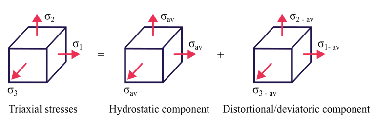
The hydrostatic stress is defined simply as the average of principal stresses as shown below:

$$\sigma_m = \frac{\sigma_1 + \sigma_2 + \sigma_3}{3} \tag{6}$$

Hydrostatic stress is an invariant, meaning its magnitude does not depend on the coordinate system or the orientation of the material element. In other words, if an element subjected to stresses in multiple directions is rotated in space, the hydrostatic stress value remains unchanged. It is a type of stress that changes only the volume of the material in the elastic state, causing expansion or contraction, while the shape of the material remains the same. For example, imagine a cube whose size changes but whose shape is preserved.

To analyze the stress components that contribute to yielding and cause plastic deformation, hydrostatic stress must be excluded. The remaining component, which alters the shape of the material, is known as the distortional stress or deviatoric stress. It is calculated by subtracting the hydrostatic stress component from the principal stress, as shown in Equation 7.

$$ \sigma_{deviatoric} = \begin{bmatrix} \sigma_1 – \sigma_m & 0 & 0 \\ 0 & \sigma_2 – \sigma_m & 0 \\ 0 & 0 & \sigma_3 – \sigma_m \end{bmatrix} \tag{7} $$

The strain energy per unit volume of the material, containing both volumetric and distortional energy, could be stated as a function of principal stresses and the Poisson ratio, shown by Equation 8.

$$u = \frac{1}{2E} \left( \sigma_1^2 + \sigma_2^2 + \sigma_3^2 – 2\nu (\sigma_1 \sigma_2 + \sigma_2 \sigma_3 + \sigma_3 \sigma_1) \right) \tag{8}$$

The volumetric strain energy could be calculated if the hydrostatic stresses would be substituted in the above equation for $\sigma_1$, $\sigma_2$, and $\sigma_3$, calculated by Equation 9.

$$u_v = \frac{3 \sigma_m^2}{2E} (1 – 2\nu) \tag{9}$$

Thus, the distortional strain energy per unit volume is obtained in Equation 10 by subtracting the volumetric strain energy per unit volume from the total strain energy per unit volume.

$$u_d = u – u_v = \frac{1+\nu}{3E} \left[ \frac{(\sigma_1-\sigma_2)^2+(\sigma_2-\sigma_3)^2+(\sigma_3-\sigma_1)^2}{2} \right] \tag{10}$$

For the specimen under uniaxial tensile test ($\sigma_1 = \sigma_Y,\ \sigma_2 = \sigma_3 = 0$), the distortional energy becomes as:

$$u_d = \frac{1+\nu}{3E} \sigma_Y^2 \tag{11}$$

Hence, the maximum distortion energy criterion states that as long as the distortion energy of the component exerted to combined loading is lower than the distortion energy of the specimen at yield, the material is safe.

$$( u_d )_{\text{component}} < ( u_d )_{\text{test specimen}} \tag{12}$$

$$\frac{1+\nu}{3E} \left[ \frac{(\sigma_1 – \sigma_2)^2 + (\sigma_2 – \sigma_3)^2 + (\sigma_3 – \sigma_1)^2}{2} \right] < \left( \frac{1+\nu}{3E} \sigma_Y^2 \right) \tag{13}$$

This criterion provides a single scalar value, known as the equivalent stress or von Mises stress, which is advantageous for assessing yielding in a component under multiaxial loading, based on the yield limit derived from a uniaxial test specimen.

$$\sigma_{\text{von-Mises}} = \frac{1}{\sqrt{2}} \left[ (\sigma_1 – \sigma_2)^2 + (\sigma_2 – \sigma_3)^2 + (\sigma_3 – \sigma_1)^2 \right]^{\frac{1}{2}} < \sigma_Y \tag{14}$$

The von Mises equivalent stress, originally expressed in terms of principal stresses, can be reformulated using the x, y, and z components of a three-dimensional state of stress, as shown in Equation 15:

$$\sigma_{\text{von-Mises}} = \frac{1}{\sqrt{2}} \left[ (\sigma_x – \sigma_y)^2 + (\sigma_y – \sigma_z)^2 + (\sigma_z – \sigma_x)^2 + 6\left( \tau_{xy}^2 + \tau_{yz}^2 + \tau_{zx}^2 \right) \right]^{1/2} \tag{15}$$

Von Mises in plane stress

For plane stress, where an element subjected to biaxial loading, the von Mises stress is reduced to Equations 16-17:

$$\sigma_{\text{von-Mises}} = \left[ \sigma_1^2 – \sigma_1 \sigma_2 + \sigma_2^2 \right]^{1/2} \tag{16}$$

$$\sigma_{\text{von-Mises}} = \left[ \sigma_x^2 – \sigma_x \sigma_y + \sigma_y^2 + 3\tau_{xy}^2 \right]^{1/2} \tag{17}$$

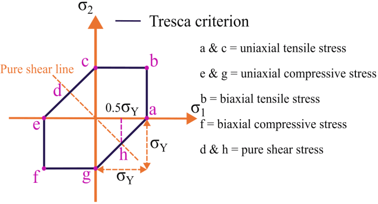
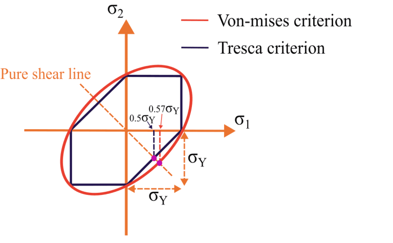
Equation 16, in the case of plane stress, forms an ellipse that overlaps with the Tresca hexagon, as shown in Figure 3.

When comparing the maximum distortion energy and maximum shear stress criteria, both predict the same results at the six points corresponding to pure tensile and compressive stresses. However, for all other stress states, the maximum shear stress criterion is more conservative, predicting a lower yield limit (i.e., yielding occurs earlier).

Yield criteria of von-mises (maximum distortion energy) and tresca (maximum shear) in combined laoding in plane stress
Figure 3 - Von-mises and Tresca yield criteria in plane stress
Yield criteria of von-mises (maximum distortion energy) and tresca (maximum shear) in combined laoding in plane stress
Figure 3 - Von-mises and Tresca yield criteria in plane stress
Yield criteria of von-mises (maximum distortion energy) and tresca (maximum shear) in combined laoding in plane stress
Figure 3 - Von-mises and Tresca yield criteria in plane stress

A particularly interesting state of stress is the pure shear (torsion) test, in which the normal stresses are zero ($\sigma_x = \sigma_y=0$). By substituting zero normal stresses into Equation 17, and setting the resulting von Mises stress equal to the yield stress from the uniaxial tensile test, the critical shear yield value for the pure shear case can be calculated:

$$ (\sigma_{\mathrm{von\text{-}Mises}})_{\text{pure shear}}
= [\,\sigma_x^2 – \sigma_x\sigma_y + \sigma_y^2 + 3\,\tau_{xy}^2\,]^{1/2}
= \sqrt{3}\,\tau_{xy} \le \sigma_Y \tag{18} $$

$$ (\tau_{xy})_{\text{pure shear}}
\le \frac{\sigma_Y}{\sqrt{3}}
= 0.577\,\sigma_Y \tag{19} $$

The predicted pure shear yield value is $0.5\sigma_Y$ according to the Tresca criterion, and $0.577\sigma_Y$ according to the von Mises criterion. It has been reported that the shear yield strength predicted by the von Mises criterion—which is less conservative than Tresca—matches the yield strength of ductile materials under pure torsion tests more accurately.

The yield criteria theories of maximum shear stress and von Mises create yield surfaces within a three-dimensional principal stress coordinate system. To understand their formation, it is important to know the space diagonal and the pi-plane.

Consider a cube element placed at the origin of the principal stress coordinate system (Figure 4-a). The space diagonal is the cube’s diagonal passing through the origin. Yield surfaces are formed by extruding yield curves along this space diagonal. This diagonal forms equal angles with all three principal stress axes, meaning points on it represent hydrostatic stress states where the stress components are equal ($\sigma_1 = \sigma_2 = \sigma_3 = 0$).

The plane perpendicular to the space diagonal at the origin is called the pi-plane (Figure 4-b). Since the space diagonal and pi-plane intersect only at the origin, stress vectors on the pi-plane other than the origin are purely deviatoric (distortional), with zero hydrostatic stress. Using the pi-plane and space diagonal, any stress state can be expressed as a combination of deviatoric stress (in the pi-plane) and hydrostatic stress (along the space diagonal). For example, point A in Figure 4-b can be represented as the sum of its deviatoric component (A-deviatoric) and hydrostatic component (A-hydrostatic). Therefore, by obtaining the yield curve on the pi-plane, the full yield surface in the principal stress coordinate system can be generated by extruding this curve along the space diagonal, as shown in Figure 4-c.

Yield criteria in space: a) space diagonal for a cube element, b) Hydrostatic and distortional components of stress in space diagonal and pi-plane, c) Von-mises and Tresca surfaces in the space
Figure 4 - Yield criteria in space: a) space diagonal for a cube element, b) Hydrostatic and distortional components of stress in space diagonal and pi-plane, c) Von-mises and Tresca surfaces in the space

The projection of the yield surfaces onto the pi-plane forms closed curves: a hexagon for the maximum shear stress theory (Figure 5-a) and a circle for the von Mises theory (Figure 5-b). The axes on the pi-plane, $\sigma_1’$, $\sigma_2’$ and $\sigma_3’$, are the projections of the principal stress axes $\sigma_1$, $\sigma_2$ and $\sigma_3$.

Imagine a cube like the one in Figure 4-a with a side length 1 and a space diagonal length of $\sqrt{3}$. Therefore, the angle between the space diagonal and each principal axis satisfies $\cos\theta = \frac{1}{\sqrt{3}}$, and the angle between any principal axes and the pi-plane satisfies $\cos\theta = \sqrt{\frac{2}{3}}$. Consequently, a point on the first principal axis with value $\sigma_1$ projects onto the $\sigma_1’$ axis on the pi-plane with length $\sqrt{2/3}\sigma_1$. Similarly, the maximum shear stress at yield ($\sqrt{2/3}\sigma_Y$) in uniaxial tension and compression along the principal axes projects onto the pi-plane as points a and b in Figure 5-a, both at length $\sqrt{2/3}\sigma_Y$. Pure shear points, labeled c in Figure 5-a, project with length $\sqrt{1/2}\sigma_Y$.

In von Mises theory, the yield curve is a circle with radius $\sqrt{2/3}\sigma_Y$, which coincides with the Tresca hexagon at uniaxial tension and compression points but exceeds it at shear points, as shown by the dashed line in Figure 5-b. Both the Tresca hexagon and von Mises circle are symmetric if the material is isotropic, indicating equal yield values in tension and compression.

 
(a) maximum shear theory (tresca hexagon) in pi-plane, (b) maximum distortion theory (von-mises) in pi-plane
Figure 5 - Projection of yield criteria in pi-plane: a) Tresca surface, b) Tresca and Von-mises surfaces
(a) maximum shear theory (tresca hexagon) in pi-plane, (b) maximum distortion theory (von-mises) in pi-plane
Figure 5 - Projection of yield criteria in pi-plane: a) Tresca surface, b) Tresca and Von-mises surfaces
(a) maximum shear theory (tresca hexagon) in pi-plane, (b) maximum distortion theory (von-mises) in pi-plane
Figure 5 - Projection of yield criteria in pi-plane: a) Tresca surface, b) Tresca and Von-mises surfaces
Yield criteria for brittle materials

The most well-known criteria for brittle materials are Maximum-Normal-Stress criterion and Mohr’s Criterion.

Maximum Normal Stress

The Maximum Normal Stress criterion, also known as the Coulomb criterion, states that a component is safe as long as the normal stresses within it remain below the ultimate strength determined from a uniaxial tensile test. In other words, the principal stresses, which represent the maximum normal stresses in the component, must be below the ultimate strength.

$$|\sigma_{1}|_{\text{component}} < |\sigma_{\text{ultimate}}|_{\text{test specimen}}\tag{20}$$

$$|\sigma_{2}|_{\text{component}} < |\sigma_{\text{ultimate}}|_{\text{test specimen}}\tag{21}$$

The above condition forms a rectangle on a coordinate system with the principal stresses as ordinates. The major drawback of this criterion is that it overlooks the difference between ultimate strengths in tension and compression, whereas brittle materials often exhibit greater compressive resistance.

Yield criterion based on normal stress theory for brittle material-important for FEA simulations of brittle materials
Figure 6 - Maximum-normal stress criterion in plane stress
Yield criterion based on normal stress theory for brittle material-important for FEA simulations of brittle materials
Figure 6 - Maximum-normal stress criterion in plane stress
Yield criterion based on normal stress theory for brittle material-important for FEA simulations of brittle materials
Figure 6 - Maximum-normal stress criterion in plane stress

Mohr’s Criterion

For a brittle material with different ultimate strengths in tension and compression, the Mohr circles for tension and compression can be drawn as shown below. The material is safe as long as the principal stresses of the component under combined loading—whether both positive or both negative—fall within the Mohr circle of the tested specimen.

The conditions above form two rectangles of different sizes on a coordinate system with the principal stresses as ordinates.

Additionally, based on the shear yield strength from a torsion test, the corresponding Mohr circle for pure shear can be drawn. As long as the Mohr circle of the component under combined loading falls within the pure shear circle, the material is also considered safe. The superposition of these three circles creates an envelope that defines a safe zone. Mohr’s criterion states that if the stress state of a component fits within this envelope, the component is safe. However, the shape of the envelope depends on the ultimate strengths from uniaxial tensile, compressive, and torsion tests. For cases where the principal stresses have different signs, the principal stress diagram can be completed by identifying the points where Mohr’s circles are tangent to the envelope and plotting these points on the principal stress diagram.

Mohr circles associated to Mohr’s stress criterion for brittle materials
Figure 7 - Mohr circles associated to Mohr’s stress criterion for brittle materials
Mohr circles associated to Mohr’s stress criterion for brittle materials
Figure 7 - Mohr circles associated to Mohr’s stress criterion for brittle materials
Mohr circles associated to Mohr’s stress criterion for brittle materials
Figure 7 - Mohr circles associated to Mohr’s stress criterion for brittle materials
Yield criteria for brittle materials in plane stress based on Mohr's stress theory and ultimate tensile and compressive stress-useful for complex FEA simulations of brittle materials
Figure 8 - Mohr’s stress criterion in plane stress
Yield criteria for brittle materials in plane stress based on Mohr's stress theory and ultimate tensile and compressive stress-useful for complex FEA simulations of brittle materials
Figure 8 -Mohr’s stress criterion in plane stress
Yield criteria for brittle materials in plane stress based on Mohr's stress theory and ultimate tensile and compressive stress-useful for complex FEA simulations of brittle materials
Figure 8 - Mohr’s stress criterion in plane stress

In the end, it needs to be noted that the integration of yield criteria into CAE workflows transforms empirical test data into powerful predictive tools. By applying von Mises or Tresca theories, engineers can confidently assess complex load scenarios while maintaining traceability to fundamental material properties. This approach balances computational efficiency with physical accuracy – a critical requirement when simulating nonlinear material behavior or optimizing weight-critical designs. As CAE systems increasingly handle multiphysics simulations, robust implementation of these failure criteria ensures virtual prototypes accurately mirror real-world material response, enabling safer and more innovative engineering solutions.

For information about Mohr’s circle, please have a look at : Mohr’s Circle blog

Picture of Amir Abdi, PhD
Amir Abdi, PhD

Amir Abdi holds a PhD in Mechanical Engineering from KTH Royal Institute of Technology, specializing in heat transfer improvement in latent thermal energy storage. He has two years of experience as a CAE Engineer at Scania’s Industrial Operations Asia division and currently works as a Climate Engineer at Envirotainer Engineering AB. Amir’s professional interests include structural mechanics, finite element analysis (FEA), computational fluid dynamics (CFD), and advanced heat transfer. His background combines hands-on engineering experience with in-depth research, enabling him to tackle complex industrial and technological challenges in energy and climate control systems.

Scroll to Top