
Miles Equation: A Practical Guide to SDOF Random Vibration Response
Key Takeaways
- The Miles equation estimates the overall GRMS acceleration of a single-degree-of-freedom (SDOF) system from just three numbers: the natural frequency $f_n$, the amplification factor $Q$, and the input PSD level $P$ at $f_n$.
- It assumes a flat white-noise input from 0 to infinity Hz and light damping. As a screening rule of thumb, it tends to work when the input PSD is flat within ±1 octave of the natural frequency — but that is not an accuracy guarantee.
- For shaped spectra, band edges and measured data, the General Method is the better tool. Multiplying the input PSD by the power transmissibility captures what Miles ignores; in our examples the Miles error reaches about 24%.
- GRMS is a 1σ value. Designers often start from a 3σ equivalent static load, and real multi-mode structures need FEA modal results with proper participation factors and modal combination.
Table of Contents
- Key Takeaways
- Introduction
- What Is the Miles Equation?
- Q, Damping and Transmissibility
- Assumptions and the One-Octave Rule
- Worked Example: NAVMAT P-9492 Input
- Miles Equation for Force Input
- Better Than Miles: The General Method
- From GRMS to Design Loads
- Using the Miles Equation Alongside FEA
- Strengths and Limitations
- Conclusion
- FAQ
- References
Introduction
A test specification lands on your desk: 6 GRMS random vibration, 20–2000 Hz, applied to each of three axes in turn. Before anyone builds an FEA model, the first question is simple — how hard will this component actually shake at its resonance? For more than seventy years, engineers have answered that question on the back of an envelope with the Miles equation.
Published by John W. Miles in 1954, the equation turns a natural frequency, a damping estimate and one PSD value into an overall response acceleration. It is fast, it is intuitive, and it is still written into test procedures, design handbooks and component specifications across aerospace, automotive and electronics.
It is also easy to misuse. This guide explains where the Miles equation comes from, what each variable means, the assumptions hiding behind it, and exactly when you should switch to the more accurate General Method. If you need a refresher on the input side first, read our guide on what GRMS means in random vibration.
What Is the Miles Equation?
The Miles equation is a closed-form expression that estimates the overall root-mean-square (GRMS) acceleration response of a lightly damped single-degree-of-freedom system excited at its base by random vibration. It assumes the input power spectral density is flat (white noise), so the response depends only on the natural frequency, the amplification factor Q, and the PSD level at the natural frequency.
The Miles Equation Formula and Its Variables
For an SDOF system subjected to a base-input acceleration PSD, the Miles equation gives the overall response acceleration as:
$$\ddot{x}_{GRMS} = \sqrt{\frac{\pi}{2}\, f_n\, Q\, P}$$
- $\ddot{x}_{GRMS}$ — overall RMS acceleration response of the mass, in g
- $f_n$ — natural frequency of the SDOF system, in Hz
- $Q$ — amplification (quality) factor, $Q = 1/(2\zeta)$, where $\zeta$ is the viscous damping ratio
- $P$ — input acceleration PSD level at $f_n$, in g²/Hz
The result is an RMS value, which equals the standard deviation (1σ) of any zero-mean response. Notice the square-root scaling: doubling the PSD level raises the response by only 41%, while doubling Q (halving the damping) does the same. That scaling is exactly why the Miles equation is so useful for quick sensitivity checks.
What the RMS alone does not tell you is the response bandwidth, the rate of peaks, the fatigue damage or the largest peak in a test. Turning it into exceedance probabilities additionally requires a Gaussian response, which in turn requires Gaussian excitation.
Where the Miles Equation Comes From
For a stable, linear time-invariant system driven by a stationary, zero-mean random input, the mean-square response equals the integral of the input PSD multiplied by the squared transmissibility (any nonzero mean is handled separately). If the input PSD is a constant $P$ from 0 Hz to infinity, $P$ moves outside the integral and only the area under the power transmissibility curve remains:
$$\begin{aligned} \ddot{x}_{GRMS}^2 &= \int_0^\infty |H(f)|^2\, P\, df \\ &= P\, f_n \int_0^\infty |H(\rho)|^2\, d\rho \\ &\approx \frac{\pi}{2}\, f_n\, Q\, P \end{aligned}$$
The exact area under the SDOF absolute-acceleration power transmissibility is $\frac{\pi}{2}\left(Q + \frac{1}{Q}\right)$ (equivalently $\frac{\pi}{2}Q\,(1 + 4\zeta^2)$). Dropping the $1/Q$ term gives the Miles equation, so Miles is a light-damping approximation even for ideal white noise: at $Q = 10$ the exact mean square is 1% higher and the exact RMS only about 0.5% higher. Everything that follows — its accuracy, its failure modes, and its alternatives — is a consequence of that step and of pulling $P$ outside the integral.
Understanding Q, Damping and Transmissibility
Q is the most influential and the least certain input to the Miles equation. It is the quality factor, defined from the viscous damping ratio as $Q = 1/(2\zeta)$, and for light damping it is approximately equal to the resonant amplification. A structure with 5% critical damping has $Q = 10$; one with 2.5% damping has $Q = 20$. The transmissibility curves below show why Q matters so much.

Figure 1. SDOF base-excitation transmissibility for Q = 1, 2 and 10. At $f = f_n$ the transmissibility is $\sqrt{1 + Q^2}$ (10.05, 2.24 and 1.41), close to Q only for light damping; all curves cross unity at $f = \sqrt{2}\, f_n$, and isolation begins above that frequency.
- Well below resonance ($f \ll f_n$), the response approaches the input and becomes nearly independent of Q. Here a static equivalent load is usually adequate — at a frequency ratio of 0.1, dynamics barely matter.
- At resonance, the transmissibility at $f = f_n$ is exactly $\sqrt{1 + Q^2}$: 10.05 for $Q = 10$, but 2.24 for $Q = 2$ and 1.41 for $Q = 1$. The true maximum occurs slightly below $f_n$. Only for light damping is the peak approximately equal to Q. This is where dynamic effects dominate and where you want to avoid placing sensitive hardware.
- At $f = \sqrt{2}\, f_n$, the transmissibility equals 1.0 regardless of Q.
- Above $\sqrt{2}\, f_n$, the system isolates: the response is lower than the input. Designers of vibration isolators deliberately push the natural frequency low so the excitation lives on this side of the curve.
Because the Miles response scales with $\sqrt{Q}$, damping is one of the few levers you can pull without changing mass or stiffness. When no test data exist, $Q = 10$ (5% damping) is a widely used screening assumption. For printed circuit boards, Steinberg (Vibration Analysis for Electronic Equipment) gives the empirical estimate $Q \approx \sqrt{f_n}$, with $f_n$ entered numerically in Hz. Either way, treat Q as an estimate, state its source, and bound your results with a sensitivity check.
Measuring Q: Half-Power Bandwidth vs. H1 and H2 Estimators
The quickest test-based estimate of Q is the half-power bandwidth method. Read the two frequencies $f_1$ and $f_2$ where the frequency response function (FRF) magnitude falls to 0.707 of its peak (−3 dB):
$$Q \approx \frac{f_n}{f_2 - f_1}, \qquad \zeta \approx \frac{f_2 - f_1}{2 f_n}$$
The half-power method works well for narrow, well-separated peaks of a linear structure. It becomes unreliable when natural frequencies sit close together; then estimate the FRF from measured force and response signals and curve-fit the modal parameters.
Bolted joints and assemblies are a different problem: friction and micro-slip make stiffness and damping amplitude-dependent, and fitting a linear model does not remove that. Check the amplitude dependence by measuring at several excitation levels representative of service. Two classical FRF estimators are:
- $H_1(f) = G_{xy}(f) / G_{xx}(f)$ — cross-spectrum of input and output divided by the input auto-spectrum. It is consistent for a noise-free input with output noise uncorrelated with the input; noise on the input (force) channel biases its magnitude downward.
- $H_2(f) = G_{yy}(f) / G_{yx}(f)$ — output auto-spectrum divided by the cross-spectrum. It is consistent for a noise-free output with uncorrelated input measurement noise; noise on the output channel biases its magnitude upward.
- $H_v$ — usually a total-least-squares (eigenvalue) estimator that accounts for noise on both channels. A geometric mean $\sqrt{H_1 H_2}$ is sometimes used as well, but lying between $H_1$ and $H_2$ does not by itself make an estimate unbiased.
If $H_1$ and $H_2$ disagree strongly around a peak, the coherence is poor at that frequency. Investigate the cause — sensor noise, leakage and windowing, force drop-out at resonance, or nonlinearity — rather than simply adding margin to the Q you extract.
Assumptions Behind the Miles Equation and the One-Octave Rule
The Miles equation is a light-damping approximation to an idealized problem. Before trusting the number it produces, check that your case is close enough to these assumptions:
- Single degree of freedom. One dominant mode carries the response. Multi-mode structures need modal analysis (see the FEA section below).
- Linear, time-invariant, viscously damped system. Stiffness and damping do not change with amplitude, which excludes gaps, friction-dominated joints and elastomer mounts driven hard.
- White-noise base input from 0 to ∞ Hz. The input PSD is perfectly flat everywhere — an assumption that is never literally true in engineering.
- Stationary, zero-mean excitation. Gaussianity is not needed to compute the RMS; it only matters when you convert the RMS into exceedance probabilities.
- Light damping. The $\frac{\pi}{2}Q$ approximation is accurate for $Q$ of roughly 5 or more.
The One-Octave Rule of Thumb
Real test profiles have ramps, plateaus and band limits, so the white-noise assumption always fails somewhere. What helps the Miles equation is that the SDOF transmissibility filters the input: much of the response energy comes from a band around the natural frequency. That leads to a screening rule of thumb used throughout the industry:
Rule of thumb: the Miles equation is usually adequate if the input PSD is flat within ±1 octave of the natural frequency — that is, from $f_n/2$ to $2f_n$. It is a screening heuristic, not an accuracy guarantee: large input contributions outside that band can still matter, and some sloping spectra still give accurate Miles estimates.
We quantify how large the errors can get in the General Method section, using two fully defined input profiles.
Worked Example: Miles Equation on a NAVMAT P-9492 Input
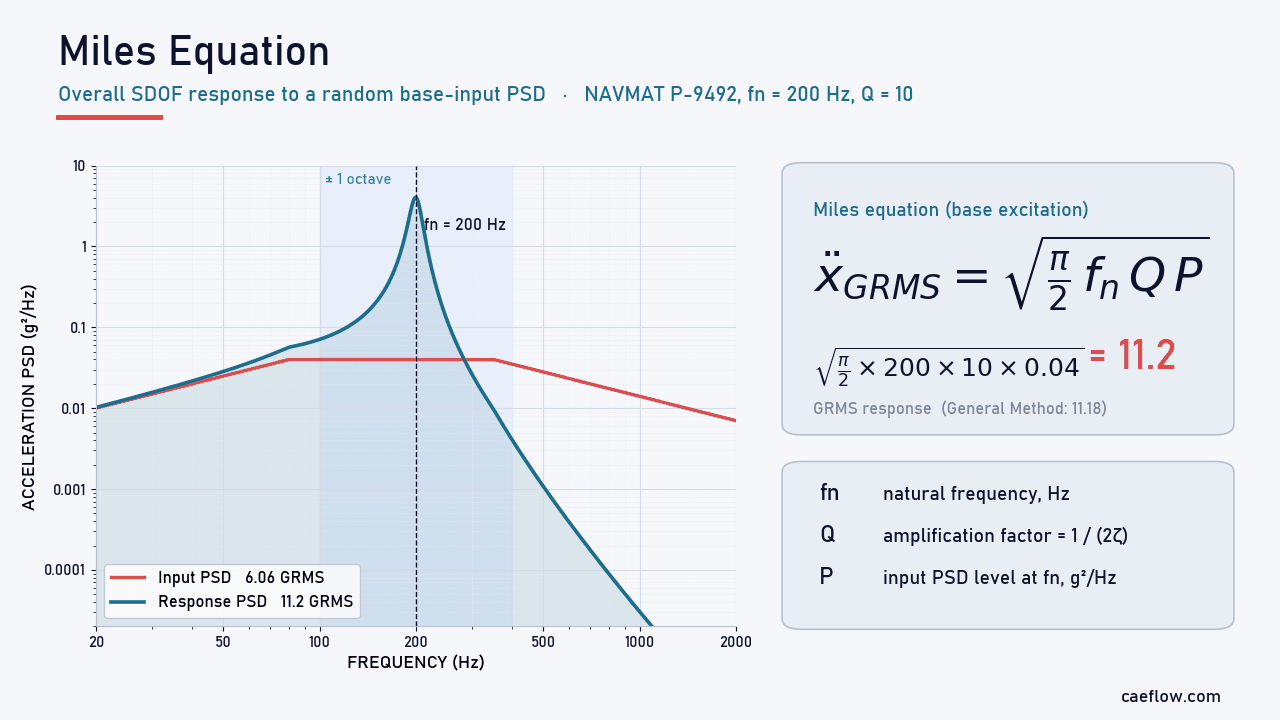
Let’s apply the Miles equation to the same NAVMAT P-9492 screening profile used in our GRMS guide, and check the answer against the General Method.
Random vibration · Worked example
SDOF response to a 6.06 GRMS NAVMAT P-9492 input
Component with $f_n = 200$ Hz and 5% critical damping, mounted on a shaker running the NAVMAT profile.
Step 1 · Inputs
Define the input PSD and the SDOF properties
The NAVMAT P-9492 profile rises in proportion to $f$ from 20 to 80 Hz, holds a 0.04 g²/Hz plateau from 80 to 350 Hz, and falls in proportion to $1/f$ to 2000 Hz. Those slopes are ±3.01 dB/octave, conventionally quoted as ±3 dB/octave; the breakpoint values with power-law (log–log) interpolation define the calculation, and the input is zero outside 20–2000 Hz.
Overall input: 6.06 GRMS. The component has $f_n = 200$ Hz and $\zeta = 0.05$, so $Q = 1/(2 \times 0.05) = 10$.
Step 2 · Validity check
Apply the one-octave rule
One octave either side of 200 Hz spans 100–400 Hz. The PSD is flat at 0.04 g²/Hz from 100 to 350 Hz but has dropped to 0.035 g²/Hz at 400 Hz, so strictly the flatness criterion is not met over the upper part of the octave. The rule of thumb suggests Miles should still be close; the integration in Step 3 is what actually establishes the accuracy.
Step 3 · Miles equation
Compute the overall response
$$\begin{aligned} \ddot{x}_{GRMS} &= \sqrt{\frac{\pi}{2} \times 200 \times 10 \times 0.04} \\ &= \sqrt{125.7} = 11.2\ \text{GRMS} \end{aligned}$$
Check: integrating the absolute-acceleration response over 20–2000 Hz (General Method) gives 11.18 GRMS, so Miles is only 0.3% high for this profile, frequency and damping. The component amplifies the 6.06 GRMS input by a factor of about 1.85.
Step 4 · Design values
Convert to peak acceleration, displacement and pseudo velocity
$$\begin{aligned} 3\sigma\ \text{peak} &= 3 \times 11.2 = 33.6\ g \\ Z_{RMS} &\approx \frac{\ddot{x}_{GRMS}\, g}{(2\pi f_n)^2} = \frac{11.2 \times 386.1}{1256.6^2} \\ &\approx 0.0027\ \text{in}\ (0.069\ \text{mm}) \\ Z_{3\sigma} &\approx 0.0082\ \text{in}\ (0.21\ \text{mm}) \\ PV &= \omega_n Z \approx 3.4\ \text{in/s RMS} \\ PV_{3\sigma} &\approx 10.3\ \text{in/s} \end{aligned}$$
Here $g = 386.1$ in/s² (use 9.81 m/s² for metric results). The displacement expression is an approximation for a lightly damped, resonance-dominated response; directly integrating the relative-displacement transfer function gives 0.0691 mm RMS, confirming it here.
This is motion relative to the base: it predicts clearance to base-fixed neighbours, while clearance between two independently moving components needs their relative motion, including correlation. The 3σ acceleration is a common starting point for an equivalent static load (see the limitations below).
The takeaway: for this particular profile, natural frequency and damping, the Miles equation agrees with a full spectral integration within 0.3%. The next sections show what happens when the conditions are less favourable.
Miles Equation for Force Input (Displacement Form)
Not every random load arrives through the base. Acoustic pressure, turbulent flow or a machine-mounted force act directly on the mass. For an SDOF system driven by a white-noise force PSD, the same integration gives the overall RMS displacement:
$$\begin{aligned} x_{RMS} &= \left[\frac{S_F}{8\zeta}\right]^{1/2} \left[\frac{1}{m}\right]^{1/4} \left[\frac{1}{k}\right]^{3/4} \\ &= \frac{1}{k}\sqrt{\frac{\pi}{2}\, f_n\, Q\, S_F} \\ &= \sqrt{\frac{S_F}{8\zeta\, m^2\, \omega_n^3}} \end{aligned}$$
Here $m$ is the mass, $k$ the stiffness, $\zeta$ the viscous damping ratio, $\omega_n = 2\pi f_n$, and $S_F$ the constant one-sided force PSD, in force²/Hz. The second form is revealing: it is simply the static compliance $1/k$ multiplied by a Miles-type term. As before, the force is assumed to be white noise from 0 to infinity Hz.
Why There Is No Acceleration Version for Force Input
For an ideal, infinite-band white-noise force, the Miles approach cannot give the acceleration response — only displacement or velocity. Above resonance, the acceleration per unit force of an SDOF system does not roll off; it flattens out at $1/m$. Integrating a constant PSD times a constant transmissibility out to infinite frequency gives an infinite mean square.
Displacement and velocity transmissibilities decay above resonance, so their integrals converge. A real, finite-band force produces a finite acceleration response: define the actual frequency band of the load and use the General Method or a frequency-response analysis in FEA.
Better Than Miles: The General Method
As described by T. Irvine, the General Method — sometimes called the “Better than Miles Equation” — solves the same SDOF problem without assuming a flat input. Instead of pulling P outside the integral, it multiplies the actual input PSD by the power transmissibility at every frequency and integrates the result. This is the method most FEA post processor and fatigue solver use for the durability calculation.

Figure 2. General Method: the input PSD multiplied by the power transmissibility $|H|^2$ gives the response PSD; integrating it yields 11.18 GRMS for $f_n = 200$ Hz and $Q = 10$.
The response PSD and the overall response are:
$$\begin{aligned} X_{PSD}(f) &= |H(\rho)|^2\, Y_{PSD}(f) \\ |H(\rho)|^2 &= \frac{1 + (2\zeta\rho)^2}{(1 - \rho^2)^2 + (2\zeta\rho)^2} \\ \ddot{x}_{GRMS}(f_n, \zeta) &= \sqrt{\sum_{i=1}^{N} |H(\rho_i)|^2\, Y_{PSD}(f_i)\, \Delta f_i} \\ \rho_i &= f_i / f_n \end{aligned}$$
$Y_{PSD}$ is the input PSD, $X_{PSD}$ the response PSD, and $\Delta f_i$ the frequency step. Arbitrary PSDs are generally integrated numerically (some special spectral shapes admit analytical integration), and the calculation is a few lines in Python, MATLAB or a spreadsheet:
- Interpolate the input PSD onto a fine, log-spaced frequency grid (use log–log interpolation between breakpoints). A useful starting resolution is at least ten points inside the half-power bandwidth $f_n/Q$; then refine the grid and check that the result has converged.
- Compute the power transmissibility $|H(\rho)|^2$ at every grid point.
- Multiply to obtain the response PSD.
- Integrate over frequency using the actual (non-uniform) frequency coordinates, and take the square root.
- Repeat for a sweep of natural frequencies to build a Vibration Response Spectrum (VRS) — the random-vibration counterpart of a shock response spectrum.
How Large Is the Miles Equation Error?
To see when the rule of thumb matters, we computed the ratio of the Miles estimate to the General Method result for $Q = 10$ across natural frequencies from 40 to 2000 Hz, for two inputs that are both zero outside 20–2000 Hz and interpolated log–log between breakpoints:- NAVMAT P-9492 — as defined in the worked example.
- Shaped PSD — 0.005 g²/Hz floor from 20 to 125 Hz; +12 dB/octave ramp from 0.005 g²/Hz at 125 Hz to 0.08 g²/Hz at 250 Hz; 0.08 g²/Hz plateau from 250 to 400 Hz; −12 dB/octave ramp down to 0.005 g²/Hz at 800 Hz; 0.005 g²/Hz floor from 800 to 2000 Hz.

Figure 3. Ratio of the Miles estimate to the General Method result (Q = 10). NAVMAT P-9492 stays within ±5% except near the 2000 Hz band edge (+17%); the shaped PSD (0.005 g²/Hz floor with ±12 dB/octave ramps to a 250–400 Hz plateau) ranges from about 24% low to 18% high.
- NAVMAT P-9492: Miles stays within about ±5% over most of the band. The exception is the 2000 Hz band edge, where it over-predicts by about 17% because it assumes the input continues beyond 2000 Hz.
- Shaped PSD, $f_n$ = 125 Hz (start of the ramp): Miles under-predicts by about 12%, because the ramp and plateau just above $f_n$ still pass through the resonance skirt.
- Shaped PSD, $f_n \approx 800$ Hz (above the plateau): Miles under-predicts by about 24%. The large input energy on the plateau passes through quasi-statically ($|H| \approx 1$ below resonance), and Miles ignores it completely.
- Shaped PSD, $f_n$ = 2000 Hz (band edge): Miles over-predicts by about 18%. This result depends on the floor: without the 0.005 g²/Hz floor, the same comparison would show Miles about 65% low — a reminder that every breakpoint matters.
In short, the Miles equation is not conservative by default. It can err in either direction, and the errors grow with steeper spectral shaping, lower Q, and natural frequencies near band edges.
When to Use Each Method
Use the Miles equation when:
- the input PSD is relatively flat within one octave of the natural frequency
- you need a quick estimate, a sanity check on FEA output, or a sensitivity study on Q
- you are screening many components early in design
Use the General Method when:
- the PSD has significant shaping — ramps, plateaus, notches or peaks
- the natural frequency falls on a PSD slope or near a band edge
- you are processing measured flight or road data with peaks and dips
- you are planning a shaker test, deriving a VRS, or feeding a fatigue damage spectrum
From GRMS to Design Loads: 3σ Peaks and Equivalent Static Loads
The Miles equation returns an RMS value, which equals the standard deviation (1σ) of a zero-mean response. If the response is Gaussian, the instantaneous acceleration lies outside ±1σ about 32% of the time and outside ±3σ only about 0.27% of the time. Note that 0.27% is the probability for an instantaneous value, not the probability of exceeding 3σ at least once during a test. To turn GRMS into a design load, engineers multiply it by a peak factor. The published conventions vary:
- 3σ — the most common assumption for the equivalent peak level (Himelblau et al., Fackler, Luhrs), with the caveat that the real response may be nonlinear and non-Gaussian
- 3σ for Space Shuttle (STS) payloads and 2σ for expendable launch vehicle payloads — historical guidance from NASA Goddard’s General Environmental Verification Specification (GEVS, 1996), not a universal current NASA rule
- 4σ — McDonnell Douglas equivalent static load practice
- 5σ — Scharton and Pankow
- nσ from the Rayleigh distribution — DiMaggio, Sako and Rubin, where n depends on the number of response cycles; Ahlin proposes a similar duration-dependent factor $C_n$
The duration-dependent approaches matter because the longer a test runs, the more likely a rare peak becomes. For a stationary, narrowband Gaussian response with $N \approx f_n T$ cycles, the leading-order estimate of the expected largest peak factor, and Davenport’s refined expected-maximum approximation, are:
$$\begin{aligned} g_p &\approx \sqrt{2 \ln N} \\ g_p &\approx \sqrt{2 \ln N} + \frac{0.5772}{\sqrt{2 \ln N}} \end{aligned}$$
For the 200 Hz component in our example, a 60-second test gives $N \approx 12{,}000$ cycles. The leading-order factor is 4.33 (about 48 g) and the refined factor 4.47 (about 50 g) — both noticeably above the 33.5 g 3σ value. These are expected-maximum estimates under the stated model, not guaranteed maxima or high-confidence design bounds; a design percentile of the maximum is higher still.
Also remember that a uniform static load of 3·GRMS does not automatically reproduce the dynamic stresses, because the dynamic deformation shape and inertia-load distribution differ from a static 1 g field. Use the convention your program or customer specifies, and state the statistical model behind it.
Relative Displacement and Pseudo Velocity
For a lightly damped, resonance-dominated response, the relative displacement is approximately $z_{RMS} \approx a_{RMS}/\omega_n^2$, with the acceleration in consistent physical units (convert g to m/s² or in/s²). This is not an exact conversion for arbitrary finite-band spectra; when accuracy matters, integrate the relative-displacement transfer function directly.
Multiplying by the angular natural frequency gives the pseudo velocity, $PV = \omega_n z$. H. Gaberson related modal velocity to stress, but the proportionality depends on the structure, material, mode and stress location — it is not a universal velocity-to-stress conversion.
Pseudo velocity is used mostly in shock analysis, and shock-severity guidelines (such as the often-quoted 100 in/s threshold) must not be used to judge random vibration: repeated cycles can cause fatigue failure at much lower levels.
Using the Miles Equation Alongside FEA
Neither the Miles equation nor the General Method replaces a finite element analysis. Real structures have many modes, and an SDOF model cannot tell you where the stress concentrates. What these methods do is make modal results far more useful, and give you an independent check on solver output.
Modal Analysis + General Method
- Run an FEA modal analysis to obtain natural frequencies, mass-normalized mode shapes and the participation factors (effective masses) for the excitation direction.
- For each significant mode, compute the modal response PSD from the input PSD and the modal transfer function (the General Method applied per mode, scaled by the participation factor), then recover responses and stresses at the locations of interest from the mode shapes and modal stresses. Frequencies and Q alone cannot predict an arbitrary nodal acceleration or stress.
- Combine the modal responses. SRSS neglects the covariance between modes and is acceptable only when those cross-terms are negligible; for closely spaced modes, include them (CQC or a full random vibration solver). Absolute acceleration also includes the base motion, not just the relative modal response.
The modal analysis runs once, and the modal results can be reused for any new PSD environment as long as the structural model is unchanged — new mass, stiffness, boundary conditions or preload require an updated modal solution. That makes the approach ideal for:
- Multiple load cases — evaluate transport, qualification and flight PSDs without re-running the modal solution
- Early trade studies — fast screening of damping assumptions and candidate environments (re-run the modal analysis whenever the design changes)
- Component screening — identify which parts need detailed analysis
- Test planning — predict the acceleration levels components will see on the shaker
- Specification development — derive component-level requirements from system-level PSDs
Sanity-Checking FEA Random Vibration Results
When an ANSYS, Nastran or Abaqus random vibration run returns a response GRMS, a Miles hand calculation for a dominant, well-separated mode (using its effective mass and the response location) should land in the same ballpark. If it is off by a factor of two, check the damping definition, the units of the input PSD (g²/Hz versus (m/s²)²/Hz), the frequency range of the analysis and the modal participation.
For large assemblies reduced with substructuring and Craig-Bampton superelements, remember that fixed-interface component modes are reduction-basis vectors, not the assembled structure’s response modes; run the check on the modes of the coupled system, in which interface motion and coupling are represented.
Preparing Measured PSD Inputs: Filtering and Decimation
If your input PSD comes from measured data rather than a specification, how you process the time history directly changes the P you feed into the Miles equation. Coupled loads analysis (CLA), for example, typically covers 0–100 Hz (up to 150 Hz for some small launch vehicles, per the ECSS Spacecraft Mechanical Loads Analysis Handbook) — typical ranges, not universal limits — while flight accelerometers are sampled far higher to capture shock. Good practice includes:
- Anti-alias before downsampling. A low-pass cutoff below the new Nyquist frequency (for example 0.8 × Nyquist) is not enough by itself: specify the transition band and make sure the attenuation is adequate at every frequency that would alias.
- Keep filtering and leakage separate. Recursive IIR filters such as a 6th-order Butterworth are common in the time domain, and a Butterworth filter is about −3.01 dB at its cutoff whatever its order. But neither time- nor frequency-domain filtering inherently eliminates spectral leakage — leakage belongs to spectral estimation (record length, windowing), and finite records add their own edge effects.
- Mind the phase for transients. A Butterworth filter’s nonlinear phase can alter transient peaks and shock response spectra, depending on the signal and the filter; it does not affect a single-channel stationary output PSD, which depends only on the filter magnitude. Forward–backward filtering gives zero phase but squares the magnitude response (about −6.02 dB at the original cutoff) and introduces its own edge considerations.
- Band-to-PSD conversion. Band RMS² divided by the bandwidth (upper minus lower frequency) gives the band-averaged PSD exactly only for an ideal rectangular bandpass filter; real filters require their equivalent noise bandwidth.
- Keep the frequency range honest. Truncating high frequencies can hide high-cycle fatigue damage in secondary structure and electronics, so filter only when you can justify it.
Strengths and Limitations of the Miles Equation
The Miles equation earns its place in every vibration engineer’s toolbox, but it should never be the last word.
Strengths:
- Closed-form and instant — no software or integration needed
- Makes the sensitivity to $f_n$, $Q$ and $P$ obvious through its square-root scaling
- Often accurate when the input is flat around the natural frequency (0.3% in our NAVMAT example)
- An excellent independent check on FEA random vibration results
Limitations:
- Assumes white noise from 0 to infinity Hz, which never exists in practice
- Ignores quasi-static input energy below resonance and truncation at band edges
- Limited to a single linear mode with viscous damping, and approximate even then (light damping)
- Cannot give an acceleration response for ideal infinite-band white-noise force input
- Returns an RMS (1σ) value — peak factors, fatigue and non-Gaussian effects must be handled separately
Conclusion
The Miles equation distills random vibration into a single, memorable line: the response GRMS equals $\sqrt{\frac{\pi}{2} f_n Q P}$. Used within its assumptions — one dominant mode, light damping and an input that is reasonably flat around the natural frequency — it can match a full spectral integration closely: within 0.3% in our NAVMAT example.
Outside those conditions it missed by up to about 24% in our shaped-PSD example, in either direction. The fix is not complicated: multiply the real input PSD by the power transmissibility and integrate. Use the Miles equation to think, the General Method to calculate, and FEA — with proper participation factors and modal combination — to capture the full structure. And always state the statistical model and peak factor you use to turn GRMS into a design load.
FAQ: Practical Questions About the Miles Equation
What is the Miles equation used for?
The Miles equation estimates the overall RMS acceleration (GRMS) of a single-degree-of-freedom system excited by a random base-input PSD. Engineers use it for quick response estimates, component screening, test planning and sanity checks on FEA random vibration results, using only the natural frequency, the amplification factor Q and the PSD level at resonance.
What is Q in the Miles equation?
Q is the quality factor, defined from the viscous damping ratio as $Q = 1/(2\zeta)$, so 5% damping gives $Q = 10$. For light damping it is approximately the resonant amplification; exactly, the base-excitation transmissibility at $f = f_n$ is $\sqrt{1 + Q^2}$. Without test data, $Q = 10$ is a common screening assumption, and Steinberg’s empirical $Q \approx \sqrt{f_n}$ ($f_n$ in Hz) is often used for circuit boards. Measure it with the half-power bandwidth method or an FRF curve fit when possible.
When is the Miles equation not valid?
It becomes inaccurate when the input PSD is not flat within one octave of the natural frequency, when the natural frequency is near a band edge, when a large share of the input energy lies below resonance, or when the structure is nonlinear or multi-modal. In those cases use the General Method or an FEA random vibration analysis; the Miles error can exceed 20% in either direction.
Can the Miles equation be used for multi-degree-of-freedom systems?
Not directly. For a multi-degree-of-freedom structure, first obtain the modes from an FEA modal analysis, then apply the Miles equation or the General Method to each significant mode and combine the modal responses (for example by SRSS). A dedicated random vibration solver is preferred when modes are closely spaced.
What is the difference between the Miles equation and the General Method?
The Miles equation assumes a flat white-noise input and uses a single PSD value at the natural frequency. The General Method multiplies the actual input PSD by the SDOF power transmissibility at every frequency and integrates the result, so it handles ramps, plateaus, peaks and band limits. The two agree when the input is flat around the natural frequency.
References (clickable):
- Miles, J. W. (1954). On structural fatigue under random loading. Journal of the Aeronautical Sciences, 21(11), 753–762.
- Irvine, T. Vibrationdata tutorials: the Vibration Response Spectrum, SDOF response to base-input and force PSDs, the “Better than Miles Equation”, and digital filtering.
- Steinberg, D. S. (2000). Vibration Analysis for Electronic Equipment (3rd ed.). Wiley.
- Davenport, A. G. (1964). Note on the distribution of the largest value of a random function with application to gust loading. Proceedings of the Institution of Civil Engineers, 28(2), 187–196.
- Gaberson, H. A., & Chalmers, R. H. (1969). Modal velocity as a criterion of shock severity. Shock and Vibration Bulletin, 40(2).
- NASA Goddard Space Flight Center (1996). General Environmental Verification Specification for STS & ELV Payloads, Subsystems, and Components (GEVS-SE).
- NASA-HDBK-7005 (2001). Dynamic Environmental Criteria. NASA Technical Standards.
- ECSS-E-HB-32-26A (2013). Spacecraft Mechanical Loads Analysis Handbook. European Cooperation for Space Standardization.
- U.S. Department of Defense (2019). MIL-STD-810H, Method 514.8: Vibration.
- Department of the Navy (1979). NAVMAT P-9492: Navy Manufacturing Screening Program.
