
Key Takeaways
Grms is the root mean square acceleration of a random vibration signal, expressed in units of g. It condenses an entire PSD into one number describing overall severity.
You calculate it by integrating the acceleration spectral density (g²/Hz) over frequency and taking the square root of the area. That area is the mean square acceleration — the variance of a zero-mean signal — not its energy.
Because PSD profiles are drawn on log–log axes, the area under a sloped segment is a power-law integral, not a trapezoid. Getting this wrong on a −3 dB/octave roll-off is worth tens of percent.
Grms is the standard way to state test severity under MIL-STD-810H, RTCA DO-160G and IEC 60068-2-64 — but two profiles with identical Grms can produce wildly different fatigue damage, so the PSD shape still governs the physics.
Table of Contents
Introduction
Ask five engineers what “6 Grms” means and you will get five answers of varying precision. Ask them to reproduce that number from the PSD it came from and the spread gets worse — usually because of how the sloped segments were integrated.
This article gives the mathematical foundation of Grms, the closed-form integration formulas for log–log PSD segments (including the singular case that breaks naive implementations), a fully worked NAVMAT P-9492 example you can check your own tools against, and the practical limits of what a single-number metric can tell you.
What Is Grms in Vibration? (Definition and Intuition)
G RMS vibration represents the root mean square of acceleration values across a frequency spectrum, expressed in gravitational units (g). It provides a single-number metric that quantifies the overall severity of random vibration environments, enabling engineers to compare test profiles and predict structural fatigue damage potential.
Understanding RMS in the Context of Random Vibration
The root mean square value isn’t arbitrary—it’s the only statistically meaningful way to characterize random processes. Unlike deterministic signals where peak values tell the whole story, random vibration contains constantly varying amplitudes across multiple frequencies simultaneously. RMS captures the effective energy content.
Here’s what makes this critical: when we say a random vibration output is 3 g RMS, we’re stating that the effective acceleration equals 3 times Earth’s gravitational acceleration (approximately 29.4 m/s²). But peak accelerations will be significantly higher—typically 3-4 times the RMS value. For a 3 g RMS signal, expect instantaneous peaks around 9-12 g.
The Gaussian distribution governs this relationship. Approximately 68% of the time, instantaneous acceleration stays within ±1σ (the RMS value). Extend to 3σ, and 99.7% of acceleration values fall within that envelope. This statistical framework directly informs how we set test limits and evaluate fatigue damage accumulation.
Grms represents the cumulative, average shaking strength over a frequency range. Think of it the way gRMS acts as the vibration equivalent of RMS voltage in electrical engineering: a sine wave might spike high, but the RMS captures the sustained power that drives fatigue and heating. That same logic applies here, making gRMS a better indicator of potential fatigue and reliability than peak acceleration alone.
If you want to know more about random vibration and its background, please have a look at our other blog: random vibration
The Difference Between Sinusoidal and Random Vibration Metrics
Comparing sine vibration (peak g) directly to random vibration (grms) without understanding crest factors leads to specification errors. Random vibrations involve multiple frequencies at once, while sine vibrations are conducted one frequency at a time. This fundamental difference means the metrics aren’t interchangeable.
In the past, most vibration was characterized in terms of sinusoids, especially at component level. Currently, most vibration is correctly understood to be random in nature and is characterized as such. This results in a demand to determine equivalence between random and sine vibration.
How to Calculate GRMS from Power Spectral Density
To calculate grms from a PSD curve, integrate the acceleration spectral density (g²/Hz) across the frequency range, then take the square root of the total area. For multi-segment PSD profiles with varying slopes, sum the area contributions from each segment before applying the square root operation.
The fundamental relationship is elegantly simple:
$GRMS = \sqrt{PSD_{Area under}}$
The input and output acceleration levels are directly related to the square root of the area under the PSD curve. This mathematical relationship means that doubling the PSD amplitude increases grms by only √2 (approximately 1.41×)—a non-intuitive result that catches many engineers off guard when performing g rms vibration calculations.
Integration Methods for Complex PSD Profiles
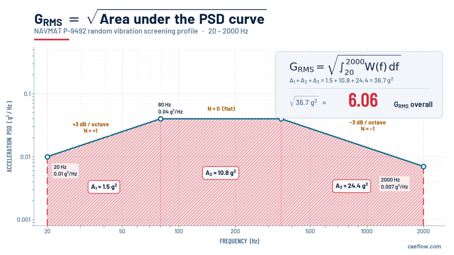
Real-world specifications rarely feature flat PSD profiles. NAVMAT P-9492 gives the power spectral density specification with an overall level of 6.0 grms, featuring +3 dB/octave and -3 dB/octave slopes with a plateau at 0.04 g²/Hz. Handling these slopes correctly requires understanding logarithmic integration.
For segments with constant dB/octave slopes, the area calculation differs from simple trapezoidal integration on linear axes. The slope in dB/octave translates to a power relationship between frequency and PSD amplitude. Most engineers find it practical to:
- Break the PSD into segments at each breakpoint frequency
- Calculate area analytically for sloped segments using the appropriate power-law formula
- Sum all segment areas
- Apply the square root to obtain grms
> ⚠️ Common Mistake: Using linear interpolation on logarithmic PSD plots. The visual appearance of a “straight line” on log-log axes represents an exponential relationship. Treating it as linear underestimates area in rising segments and overestimates in falling segments.
Practical Calculation Example with Industry-Standard Profile
The vibration profile referenced in the NAVMAT P-9492 is a 6 g RMS random 20-2000 Hz Power Spectral Density (PSD) curve. This specification has become a de facto standard for environmental stress screening and provides an excellent validation case for your calculation tools.
The profile features breakpoints at 20 Hz, 80 Hz, 350 Hz, and 2000 Hz, with slopes connecting them. When you integrate correctly, your result should match the published 6.0 grms value. If your calculation deviates by more than 1-2%, examine your slope handling and frequency resolution.
While the magnitude of the input RMS acceleration level indicates severity, the magnitudes of the input PSD levels in the regions of the structure’s resonant frequencies are far more important for predicting actual response. This insight fundamentally shapes how we approach random vibration analysis—it’s not just about the overall grms number.
How GRMS is calculated from a PSD
GRMS is the square root of the area under the acceleration PSD. Because PSD profiles are drawn on log–log axes, that area is not a trapezoid: each straight segment is a power law with its own closed-form integral. Three steps, then a worked NAVMAT P-9492 example you can edit.
Area under the PSD is the mean square acceleration
For a stationary, zero-mean random signal, integrating the acceleration spectral
density W(f) over frequency returns the variance of the signal, which is
the mean square acceleration. Take the square root and you have the RMS level, in g.
Two consequences worth internalising: the area scales with amplitude, so doubling the whole PSD raises GRMS by only √2 ≈ 1.41×, and a +6 dB shift (×4 in g²/Hz) exactly doubles it. And GRMS depends on the integration limits, so quoting a level without its bandwidth is meaningless.
A straight line on log–log axes is a power law, not a ramp
Specifications give breakpoints and slopes in dB/octave. On log–log paper a
straight segment between (f1, W1) and
(f2, W2) obeys log W = N·log f + log b,
which in exponent form is Steinberg’s Eq. 9.16:
Integrate each segment in closed form, then sum
Split the profile at every breakpoint using vertical lines only, integrate
b·fN across each segment, add the areas, and take a
single square root at the very end. Never square-root the segments individually.
Flat · N = 0
Sloped · N ≠ −1
Exactly −3 dB/oct · N = −1
The N = −1 case is a genuine singularity, not a rounding issue: the general formula divides by (N + 1). Any code that integrates PSD segments has to branch on it, and −3 dB/oct is one of the most common roll-offs in the standards, which is exactly why it bites.
NAVMAT P-9492, 20–2000 Hz
Three segments: +3 dB/oct up to the 0.04 g²/Hz plateau, flat to 350 Hz, then −3 dB/oct to 2000 Hz. Areas 1.5 + 10.8 + 24.4 = 36.7 g², and √36.7 = 6.06 gRMS. Edit any value to see the number move, or switch to linear axes to see why the segments are curves.
| Frequency (Hz) | PSD (g²/Hz) | |
|---|---|---|
| Segment | N | dB/oct | Area (g²) |
|---|---|---|---|
| 20 → 80 Hz | +1.00 | +3.0 | 1.50 |
| 80 → 350 Hz | +0.00 | +0.0 | 10.80 |
| 350 → 2000 Hz | −1.00 | −3.0 | 24.40 * |
| Σ areas = m₀ | 36.70 g² |
Linear trapezoid rule would give 7.15 gRMS — 18.0% off.
Trapezoids on a log–log plot
Do not trapezoid between breakpoints
A segment that looks like a straight line on log–log axes is
W = b·fN in linear space. Joining the breakpoints with a
straight line in linear space and taking
½(W1+W2)(f2−f1)
is exact only for N = 0 (flat) and N = +1 (+3 dB/oct), where the
log–log line really is straight in linear space too. Everywhere else the sign of
the error follows convexity: for N < 0 or N > 1 the chord sits above
the true curve and the trapezoid over-estimates; for 0 < N < 1 it
under-estimates. On NAVMAT the −3 dB/oct segment alone jumps from 24.4 to
38.8 g² (+59 %) and the overall level goes from 6.06 to
7.15 gRMS, an 18 % error you would never catch by eye.
Software Tools for G RMS Vibration Analysis
Professional g rms vibration analysis tools span FEA post-processors, dedicated vibration testing software, and accelerometer signal processing packages. Your selection depends on whether you’re analyzing simulation outputs, processing physical test measurements, or correlating between both domains.
FEA Post-Processing Capabilities
Major solvers (ANSYS, Nastran, Abaqus) include native random vibration modules that compute response PSD and grms values directly. The workflow typically involves:
- Performing modal analysis to extract natural frequencies and mode shapes
- Defining input PSD excitation at base or distributed locations
- Running random response analysis using modal superposition
- Requesting acceleration PSD output at critical locations
- Integrating response PSD to obtain grms
The critical consideration here is modal truncation. If your frequency range of interest extends to 2000 Hz but you’ve only extracted modes to 500 Hz, your g rms vibration calculation will be unconservative. Always extract modes to at least 1.5× your maximum frequency of interest.
How Grms Is Used in Random Vibration Testing
In random vibration testing, an electrodynamic shaker generates broadband excitation shaped to match a target PSD profile. Accelerometers monitor shaker vibrations during random vibration testing, and the control system continuously checks that the measured PSD and overall Grms stay within prescribed tolerances. Random vibration testing simulates real-world vibration environments by exciting multiple frequencies simultaneously instead of sweeping one tone at a time.
Common standards for random vibration testing include MIL-STD-810 and IEC 60068-2-64. These standards, along with RTCA DO-160G Section 8, define test requirements by specifying a PSD curve, an overall grms value, bandwidth, duration (often one hour per axis), and control limits. Random vibration can be broadband or narrow band depending on the environment being replicated.
A high GRMS value indicates strong vibrations that may cause damage, so test houses typically quote shaker capability in terms like “up to 40 Grms from 20–2000 Hz” for a given payload mass. The selected grms level and duration represent a target amount of in-service damage, sometimes established through fatigue damage equivalence. During the test, engineers verify channel-by-channel that the measured response on the component under test matches the input PSD within defined tolerances, adjusting or aborting if Grms drifts outside limits.
Strengths and Limitations of Using Grms
Grms is an essential but not complete descriptor of a random vibration event. Here is what it does well and where it falls short.
Strengths:
Provides a single numeric indicator of overall vibration magnitude, making it easy to compare different environments or test levels
Directly tied to PSD-based random vibration testing and analysis workflows
Supports fatigue damage equivalence methods and shaker sizing decisions
Lets you predict expect exceedance levels using probability distributions
Limitations:
Does not show how energy is distributed across frequency, so resonance effects may be hidden
Two vibration profiles with identical Grms can produce very different structural damage if one concentrates energy near the component’s natural frequencies
Does not capture short, damaging shock-like transients or non-Gaussian statistical properties (high kurtosis)
Complementary tools include detailed PSD review, time-history inspection, kurtosis analysis, and combined environment testing (vibration plus temperature). Treat Grms as a starting point for vibration analysis, not the final answer.
Conclusion
G rms vibration analysis demands precision at every step—from understanding the statistical foundation of RMS values to correctly integrating complex PSD profiles. The single-number severity metric derived from spectral density integration enables meaningful comparison across test profiles and simulation predictions, but only when calculated consistently.
Accurate grms calculation requires proper handling of logarithmic PSD slopes and appropriate frequency resolution. Software tools must be validated against hand calculations using known reference profiles before trusting automated outputs for qualification decisions. When projects involve regulatory compliance, multi-axis environments, or test-simulation correlation challenges, professional services provide validated methodologies that reduce program risk.
Your next step: validate your current g rms vibration calculation workflow by computing the NAVMAT P-9492 profile (6.0 grms, 20-2000 Hz) and comparing results across your analysis tools. Any deviation greater than 2% warrants investigation into your integration methodology. This simple validation exercise builds confidence in your random vibration analysis capabilities and prevents costly surprises during vibration testing campaigns.
FAQ: Practical Questions About Grms in Vibration
What does grms stand for?
Grms stands for “gravitational root mean square,” representing the RMS acceleration level of a vibration signal expressed in units of g (9.81 m/s²). It quantifies overall random vibration intensity across a defined frequency spectrum, serving as the primary severity metric in dynamic testing specifications.
How to calculate grms vibration?
Calculate grms by integrating the power spectral density (PSD) curve across the frequency range and taking the square root. For each PSD segment, compute the area (g²/Hz × Hz = g²), sum all segment areas, then apply the square root to obtain the final grms value.
What is the g level in vibration?
The g level in vibration refers to acceleration magnitude expressed as multiples of gravitational acceleration (1g = 9.81 m/s²). For random vibration, g levels are reported as grms values representing statistical intensity, while sinusoidal vibration uses peak g values.
What does RMS mean for vibration?
RMS (root mean square) for vibration represents the effective value of a fluctuating acceleration signal. It equals the square root of the mean of squared instantaneous values, providing a statistically meaningful single number that correlates with vibration energy and fatigue damage potential.
How does frequency range affect grms calculations?
Frequency range directly impacts grms because the calculation integrates PSD area across specified bandwidth. Wider frequency ranges typically yield higher grms values. Engineers must ensure calculation bounds match specification requirements, as truncating high-frequency content artificially reduces reported severity.
References (clickable):
- Brüel & Kjær. (2018). The frequency domain: FFT & PSD made easy [Application note]. Brüel & Kjær.
- Hottinger Brüel & Kjær (HBK). (n.d.). Knowledge base: Spectral analysis and random vibration reference articles.
- Performing Random Vibration Analysis Using Ansys Mechanical, ANSYS Learning.
- Lalanne, C. (2009). Mechanical vibration and shock analysis: Volume 3 – Random vibration (2nd ed.). Wiley.
- MathWorks. (n.d.). Power spectral density estimates using FFT.
- National Instruments. (2012). Understanding power spectral density (PSD) measurement.
- Newland, D. E. (2012). An introduction to random vibrations, spectral & wavelet analysis (3rd ed.). Dover Publications.
