Shock Response Spectrum (SRS): The Comprehensive Engineering Guide
Theory, Calculation, and Advanced FEA Implementation
Key Takeaways
Definition: SRS plots the maximum response of a series of single-degree-of-freedom (SDOF) oscillators to a transient event.
Key Application: Used for qualifying hardware against pyroshock, seismic events, and drop impacts.
Damage Potential: Correlates with yield and ultimate stress failure (Peak Response), unlike PSD which predicts fatigue.
Sampling Requirement: Accurate capture of peak amplitudes requires a sample rate at least 10x the maximum frequency of interest (often >100 kHz for pyroshock).
Primary Use: SRS is used for component qualification (determining if a part will survive a specific shock) rather than fatigue analysis.
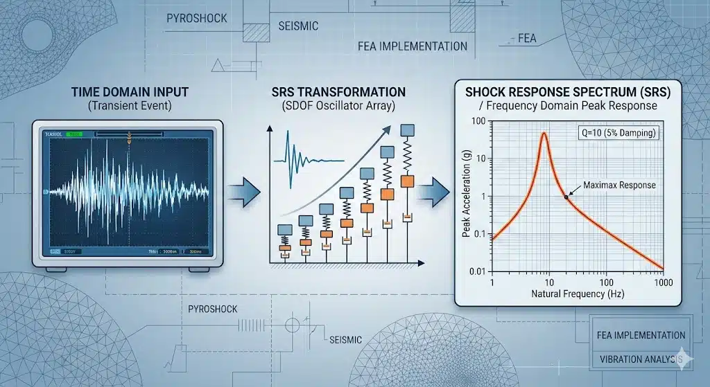
Table of Contents
What Is a Shock Response Spectrum (SRS)?
A Shock Response Spectrum (SRS) is a method to estimate the peak response of a system to the transient base motion input.
The Shock Response Spectrum (SRS) is a fundamental tool in structural dynamics that translates complex transient time-domain events into frequency-dependent peak response data.
Unlike vibration analysis methods that focus on energy distribution (like PSD) or statistical properties, the SRS specifically answers the critical engineering question: “What is the maximum response a structure will experience at each natural frequency?”
This characteristic makes the SRS invaluable for qualifying components against severe transient events such as pyroshock, drop impact, vehicle crash, and seismic excitation. The SRS focuses on damage modes like yield, buckling, and ultimate stress failure.
The response spectrum concept originated in earthquake engineering in the 1930s (von Kármán and Biot). Biot proposed that rather than analyzing the exact shape of input time histories, engineers should focus on the effect—represented by the response of SDOF oscillators. The U.S. Navy later adapted this for aerospace pyrotechnic shock in the 1960s.
Fundamental Concepts
The SDOF Oscillator Model
The SRS is built upon the single-degree-of-freedom (SDOF) oscillator model—a mass-spring-damper system subjected to base excitation. For a base acceleration input $\ddot{y}$, the equation of motion for relative displacement $z$ is:
$$\ddot{z} + 2\xi\omega_n\dot{z} + \omega_n^2z = -\ddot{y}$$
Where:
- $\xi$ is the damping ratio.
- $\omega_n$ is the natural circular frequency.
The absolute acceleration of the mass, often the primary metric of interest, is:
$$\ddot{x} = -2\xi\omega_n\dot{z} – \omega_n^2z$$
An SRS plots the peak acceleration responses of a bank of single degree-of-freedom (SDOF) spring, mass damper systems all experiencing the same base-excitation as if on a rigid massless base. Each SDOF system has a different natural frequency; they all have the same viscous damping factor. A spectrum results from plotting the peak accelerations (vertically) against the natural frequencies (horizontally).
Relative damping of 5% results in a Q of 10. An SRS plot is incomplete if it doesn’t specify the assumed Q value. This is a critical point I’ve seen engineers overlook—comparing SRS curves computed with different damping values leads to meaningless conclusions.
Frequency Domain Representation of Transient Events
A common misconception with Shock Response Spectra is that it is a frequency domain signal. In fact, the Shock Response Spectra is actually calculated from the peak time domain response of a single degree of freedom system. This distinction matters for implementation—you’re tracking peak responses in time, then plotting against frequency.
The power of SRS lies in translating raw acceleration data into design-relevant information. The graphs show a shock pulse and its Shock Response Spectra. Note that the peak on the pulse waveform is only about 17 g’s while the peak Shock value for SRS is 40 g’s. This amplification at resonance is precisely what we need to capture for qualification purposes.
SRS Calculation Methods: Algorithms and Mathematical Implementation
To calculate the SRS, the physical system is represented as several SDOF systems with increasing order of their natural frequencies, and their absolute peak response is calculated when subjected to a transient input excitation. This peak acceleration is plotted against natural frequency in a graph, which is termed as Shock Response Spectrum (SRS). The implementation details significantly impact accuracy and computational efficiency.
Recursive Digital Filter Approach
The absolute acceleration response of a SDOF oscillator is primarily used to compute the shock response spectrum. This response can be computed using discrete time methods like the recursive filtering method or the Prefilter-Smallwood method.
The Smallwood ramp invariant digital recursive filtering algorithm is the industry standard. It solves the SDOF equation efficiently using a feedback loop:
$$\ddot{x}_i = f(\ddot{x}_{i-1}, \ddot{x}_{i-2}, \ddot{y}_i, \ddot{y}_{i-1}, \ddot{y}_{i-2}, \xi, \omega_n, \Delta t)$$
Sample Rate Requirements
- General Rule: Sample rate > 10× $f_{max}$ (< 5% error).
- Pyroshock: Sample rates > 100 kHz are mandatory to capture steep rise times.
Sample rate requirements are non-negotiable for accurate results. The sample rate must be higher than 10 times the maximum frequency of the spectrum so that the error made at high frequencies is lower than 5%. For a maximum error of 1%, the sample rate should be higher than 23 times the maximum frequency of the spectrum.
💡 Pro Tip: When processing pyroshock data targeting 10 kHz analysis frequency, ensure your sample rate exceeds 100 kHz—cutting corners here produces systematically low SRS values at high frequencies.
For specific waveforms, the recursive integration method suffers from numerical approximation error in higher natural frequencies. To reduce the error of the recursive integration approach, the waveform must be discretized at higher sample rate.
Data Acquisition and Preprocessing Standards
Mechanical shock has the potential for producing adverse effects on the physical and functional integrity of material. In general, the damage potential is a function of the amplitude, velocity, and duration of the shock. Adverse effects on the materials overall integrity are magnified when shocks frequency content correspond with the material’s natural frequencies.
For pyroshock events, the sampling rates often need to exceed 100 kHz, with maximum SRS frequency limited to approximately fs/10 for adequate SDOF response resolution. Anti-aliasing filters are mandatory before digitization—this cannot be corrected in post-processing.
> 📋 Quick Reference: Data Quality Requirements
> – Pyroshock: >100 kHz sample rate, analog anti-aliasing filter
> – Drop/Impact: >10 kHz typical, capture full ring-down
> – Transportation: Match to expected frequency content, typically 5-2000 Hz range
MIL-STD-810 addresses a broad range of environmental conditions that include shock and transport shock. Reference MIL-STD-810H Method 516.8 and IEST-RP-DTE012 for detailed data acquisition requirements specific to your application.
SRS vs. PSD: What’s the Difference?
Engineers often confuse Shock Response Spectra with Power Spectral Density (PSD). They are fundamentally different tools for different environments. Read PSD blog about the random vibration
| Feature | SRS (Shock Response Spectrum) | PSD (Power Spectral Density) |
|---|---|---|
| Event Type | Transient, deterministic events (Pyroshock, Drop, Crash) |
Continuous, random vibration (Engine hum, road noise) |
| Metric | Peak Acceleration (g) vs. Frequency | Energy (g²/Hz) vs. Frequency |
| Damage Mode | Yield, Buckling, Ultimate Stress | Fatigue, Cumulative Damage |
| Duration | Milliseconds to Seconds | Minutes to Hours |
Velocity and Displacement SRS: Beyond Acceleration Response
One of the other primary benefits of the SRS is that by being in the frequency domain, converting to velocity and displacement is quite simple. And velocity is more indicative of the damage potential of a shock event than acceleration levels. This insight fundamentally changes how we assess shock severity for certain component types.
Howard Gaberson (U.S. Navy) championed the concept that dynamic stress correlates more directly with pseudo velocity than acceleration.
$$[\sigma_n]_{max} = K \rho c [v_n]_{max}$$
Where $\rho$ is density, $c$ is wave speed, and $v$ is velocity. This explains why high-G, high-frequency shocks (which have low velocity) often cause less damage than low-G, low-frequency shocks.
The pseudo velocity shock spectrum (PVSS) plot can initially make your head hurt, but when you get used to it you can fully realize its value. This is called a tripartite or four coordinate plot because it is not only providing the pseudo velocity relationship but also includes the displacement and acceleration.
For large equipment or seismic qualification where displacement-sensitive components may fail despite moderate acceleration levels, velocity SRS provides superior insight.

Shock Analysis Software Implementation: Workflow Integration
Implementing SRS in FEA workflows requires importing measured shock spectra as base excitation inputs, selecting appropriate SDOF damping values matching test conditions, and correlating analytical predictions with physical test results for model validation. The integration between test data and simulation is where many programs stumble.
Commercial Tool Considerations
An SRS is generated from a shock waveform using the following process: Specify a damping ratio for the SRS (5% is most common). Use a digital filter to model an SDOF of frequency $f_n$ and damping $\xi$. Apply the transient as an input and calculate the response acceleration waveform. Retain the peak positive and negative responses occurring during the pulse’s duration and afterward.
MATLAB’s Signal Processing Toolbox, Python libraries (scipy with custom implementations), and dedicated shock analysis software all provide SRS calculation capabilities. Key considerations include batch processing for multiple channels, import/export format compatibility, and octave spacing options.
One good tutorial is Ansys learning Response Spectrum Analysis youtube series.
FEA Model Correlation with SRS Data
The first step in evaluating shock response of a system is to perform a modal analysis to obtain natural frequencies and corresponding mode shapes of the physical system. This is a linear dynamics procedure in which stiffness and mass matrices are calculated for the system. These matrices are used to extract the eigenvalues and mode shapes.
Any transient waveform can be presented as an SRS, but the relationship is not unique; many different transient waveforms can produce the same SRS. The SRS does not contain all of the information about the transient waveform from which it was created because it only tracks the peak instantaneous accelerations.

This non-uniqueness creates the inverse problem—synthesizing time histories from SRS specifications for simulation input. Common synthesis methods include wavelets and damped sinusoids, each with trade-offs in computational efficiency and waveform characteristics.
Interpreting Results for Design
SRS interpretation requires engineering judgment. The numbers mean nothing without context.
Identify Resonances: Compare spectrum peaks against your component’s natural frequencies.
Apply Margins: Use appropriate margin factors (typically +3dB or +6dB) per qualification standards.
Mitigation Strategies:
Stiffen up structure: Shift natural resonances away from high-G conditions.
Isolate: Apply shock isolators to dampen modal velocities.
Relocate: Move sensitive components to the sections with lower displacement.
Critical Limitation: An SRS is of little use for fatigue-type damage scenarios. It tracks peak response, not cumulative damage.
Conclusion
Shock response spectrum (SRS) analysis transforms complex transient shock waveforms into frequency-dependent response data essential for component qualification—bridging the gap between raw acceleration measurements and actionable design decisions. Accurate calculation demands proper input data conditioning with sufficient sample rates, appropriate damping selection matching your test conditions, and adequate frequency resolution across your analysis bandwidth.
Interpretation requires engineering judgment beyond the computed curves. The SRS characterizes shock severity but requires synthesis for test specification development, and the non-unique relationship between time histories and spectra means multiple valid test waveforms can satisfy a single specification. Integration with FEA workflows enables predictive analysis, but only when properly correlated against physical test data.
Ready to validate your workflow? Start by processing a known reference shock pulse—like a half-sine or terminal-peak sawtooth with published analytical solutions—before applying these methods to critical qualification programs. Verification is the only way to ensure your calculated margins are real.
Frequently Asked Questions (FAQ)
What is shock response spectrum?
A Shock Response Spectrum (SRS) is a graphical presentation of a transient acceleration pulse’s potential to damage a structure. It plots peak acceleration responses of SDOF systems experiencing base-excitation, characterizing shock severity across frequency for component qualification decisions.
How is SRS shock response spectrum calculated?
Pick a damping ratio, select a frequency f, and assume a hypothetical SDOF system with that damped natural frequency. Calculate maximum instantaneous absolute acceleration experienced during or after shock exposure. Repeat for many frequencies and plot results to generate the spectrum.
What is the difference between SRS and PSD analysis?
SRS analyzes transient, deterministic shock events by tracking peak SDOF responses, while PSD characterizes stationary random vibration through frequency-domain energy distribution. Use SRS for impacts and pyroshock; use PSD for continuous random vibration environments.
Why is damping ratio important in shock response spectrum analysis?
Different damping ratios produce different SRS curves for identical shock waveforms. Zero damping produces maximum response while high damping flattens the spectrum. A 5% damping ratio (ξ=0.05) results in Q=10. Matching test conditions ensures meaningful analysis-to-test correlation.
How do you synthesize a time history from an SRS specification?
Time history synthesis involves generating waveforms matching target spectrum specifications. Common methods include summing damped sinusoids or using wavelet-based approaches. Multiple valid time histories can produce identical SRS curves due to the non-unique relationship between waveforms and spectra.
References (clickable):
- Irvine, T., “Shock and Vibration Response Spectra,” Vibrationdata.
- Smallwood, D., “An Improved Recursive Formula for Calculating Shock Response Spectra,” Shock and Vibration Bulletin, 1981.
- USNRC Regulatory Guide 1.92, Rev 3, “Combining Modal Responses and Spatial Components in Seismic Response Analysis.”
- Gaberson, H., “Shock Severity Estimation,” Sound & Vibration, 2012.

I am a senior CAE and Automation Engineer at Scania with over 8 years of hands-on experience in Finite Element Analysis (FEA). My daily work involves advanced simulations focusing on strength and durability analysis, helping design more reliable and efficient products.
Before joining Scania, I conducted research at KTH Royal Institute of Technology, where I focused on the additive manufacturing of heat exchangers. My work has been recognized internationally and published in peer-reviewed journals. You can find my publications on Google Scholar.
In June 2019, I managed to secure the funding for continuation of my PhD by receiving a grant of 3.7 MSEK from the Swedish Energy Agency on development of 3Dprineted air-PCM heat exchangers.