Frequency Response Function: Theory & Applications Guide
The Frequency Response Function (FRF) stands as a cornerstone in vibration analysis, structural dynamics, and system identification. This comprehensive guide explores how FRFs characterize the response of a system across different excitation frequencies, providing engineers with essential insights for modal analysis, structural health monitoring, and vibration troubleshooting.
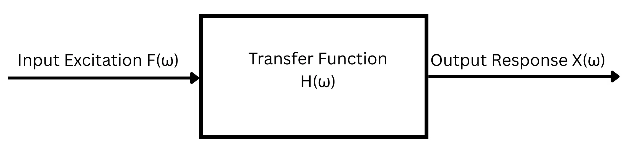
Table of Contents
What is a Frequency Response Function (FRF)?
Essentially, a Frequency Response Function (FRF) is the ratio between output (response of a structure/system) to input excitation. It is an inherent characteristic of systems and is unique to each structure.
FRF has many applications across various fields including electrical and audio engineering. However, the focus of this blog is mechanical vibration.
In mechanical vibration, we are primarily interested in how structures respond to input excitation. This excitation comes from the surrounding environment, and our goal is to understand and predict the output response. By understanding the frequency response function, we can design structures to minimize unwanted vibrations and avoid resonance, which causes excessive displacement and potentially catastrophic stress on the overall structure.
Input excitation falls primarily into two categories:
Force (load) excitation: Examples include shaft misalignment in rotating machinery, snow loading on wind turbine blades, or ocean waves impacting breakwaters.
Base excitation: Examples include earthquake ground motion affecting buildings or suspension vibration in vehicles traveling on uneven roads.
As we said above, the ratio between the response of the structure and the input is called the frequency response function. FRF is unique for each structure since it depends on mass, stiffness, and damping of a system. For a hands-on interactive exercise regarding FRF, please read our blog about sine sweep testing.
Note that as the name suggests, FRF is calculated in the frequency domain. The input can be any type. It can be random, sine, or etc. The output response can be acceleration, velocity, or displacement depending on what is measured and analyzed. We will cover those in detail later in this blog.

$$ H(\omega) = \frac{X(\omega)}{F(\omega)} \tag{1} $$
$H(\omega)$ – Frequency Response Function
$X(\omega)$ – Output Response (frequency domain)
$F(\omega)$ – Input Excitation (frequency domain)
Similar transfer functions can be developed for the velocity and acceleration responses. The above was for displacement.
Types of Input Excitation in FRF Measurements
When exciting the system for frequency response measurements, engineers typically employ:
- Force Excitation: Including impact hammers, shakers to excite structures, or operational loads
- Base Excitation: Such as earthquake simulations or vehicle suspension testing
- Broadband Excitation Signals: White noise, chirp signals, or random excitation
- Sine Wave Testing: Including sine sweep testing for detailed frequency response curves
Fundamentals of Frequency Response Analysis
Natural Frequencies and Resonance in System Dynamics
Structures vibrate at specific natural frequencies when disturbed—think of how a tuning fork rings at a particular pitch. Every bridge, building, or machine component has multiple natural frequencies that depend on its physical properties.
Resonance is what happens when external forces match these natural frequencies, causing vibrations to grow dangerously large. This amplification effect can destroy structures, which is why engineers must identify and avoid these critical frequencies [1]. One of the most famous case example is a collapse Tacoma bridge back in 1940 due to The collapse of the Tacoma Narrows Bridge was driven by wind-generated vortices that reinforced the twisting motion of the bridge deck until it failed, watch video below [2,3].
Input-Output Relationships in Dynamic Systems
Consider a single degree of freedom (SDOF) system. It is made up of mass, spring and damper, see Figure 2.
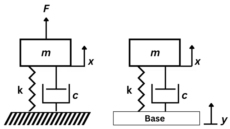
m, k and c are characteristics of the system and is unique. If we apply a base excitation at y or force input at mass, then we expect a response in terms of displacement at x.
The response has both magnitude and phase that can be different than the input. This is quite important since when we plot the FRF, we can plot the amplitude and the phase in different plots.
We will proceed with force excitation mathematical derivation, but the procedure is similar for base excitation except that we need to define relative displacement which we cover in another blog in future.
Mathematical Derivation of FRF
For a mass-spring-damper system with external force F(t), Newton’s second law gives us:
This is the frequency response function (FRF) for force excitation, expressing the complex ratio between displacement output and force input.
Amplitude and Phase Characteristics
As shown in Equation (9), the right hand of equation has both real and imaginary part. The complex-valued FRF contains two essential components:
- Magnitude (Amplitude versus Frequency): Shows amplification or attenuation at each frequency
- Phase Response: Indicates time delay between input and output signals
These characteristics help engineers understand:
- How the system amplifies or attenuates different frequency components
- Phase relationships crucial for closed-loop stability analysis
- Frequency-dependent behavior affecting system performance
Below interactive plot helps you to understand the FRF concept.
Physical Interpretation
Do the following interactive exercise for a SDOF that we discussed above, and see how the three zones changes based on different parameters.
Fast Fourier Transform and Spectral Analysis
Modern FRF estimation relies heavily on Fast Fourier Transform (FFT) algorithms to convert time-domain input and response data into the frequency domain. The process involves:
- Data Acquisition: Recording input signal and vibration response using sensors
- FFT Processing: Converting time-domain signals to frequency spectra
- Spectral Estimation: Computing power spectral densities and cross-spectra
- FRF Calculation: Using appropriate estimators (H1, H2, or Hv)
We cover FFT and estimators in another blog. For now, just note that in software like MATLAB or nCode, you have the option to convert time-domain signals from accelerometers into the frequency domain using FFT functions.
Modal Analysis and System Identification Applications
Extracting Modal Parameters from FRFs
- The whole point is to excite the structure across frequency ranges and identify peaks that reveal the system’s natural frequencies based on the input and the structural response. In other words, modal analysis transforms multiple FRFs into modal parameters such as:
Natural frequencies and damping ratios
Mode shapes and modal masses
Participation factors for each mode
This information enables:
Validation of finite element models
Design optimization for dynamic performance
Troubleshooting of vibration problems
For further information about modal analysis, please check this: FEA Modal Analysis
Frequently Asked Questions (FAQ)
What is the frequency response function and how does it describe the system?
The frequency response function (FRF) is a crucial tool in system identification that characterizes the output of a system in response to a given input frequency. It provides insights into how the system behaves across a range of frequencies, illustrating the relationship between the input signal and the output signal. This function is essential for understanding the dynamic behavior of mechanical systems and is often used in structural dynamics and vibration analysis.
How do you measure the frequency response of a system?
To measure the frequency response of a system, one typically applies a known input signal, often a sinusoidal or broadband excitation signal, and records the resulting output signal. Using techniques such as the Fast Fourier Transform (FFT), one can analyze the amplitude and phase of the system’s output across different frequencies. This data allows engineers to create frequency response curves, which illustrate how the system responds to various input frequencies.
What is the relationship between input and output signals in frequency response analysis?
In frequency response analysis, the relationship between the input and output signals is fundamental. The input signal is typically an excitation applied to the system, while the output signal is the system’s response. By analyzing how the output frequency varies with changes in the input frequency, engineers can gain insights into the system’s dynamics, including natural frequencies and resonant behavior.
Can you explain the frequency range of interest in frequency response function analysis?
The frequency range of interest in frequency response function analysis refers to the specific frequencies over which the system’s response is evaluated. This range is crucial for capturing the relevant dynamics of the system, as it may include critical frequencies where resonances occur. Selecting an appropriate frequency range ensures that the analysis can effectively identify key characteristics of the system’s behavior.
How does modal analysis relate to the frequency response of a system?
Modal analysis is a technique used to determine the natural frequencies and mode shapes of a system based on its frequency response function. By examining the system’s response at various frequencies, engineers can identify specific modes of vibration and their corresponding frequencies. This information is vital for structural dynamics and health monitoring, helping to optimize designs and predict potential failure points.
Conclusion
The Frequency Response Function remains an indispensable tool for understanding system dynamics. By mastering FRF concepts and measurement techniques, engineers can effectively characterize mechanical systems, validate analytical models, and optimize designs for superior dynamic performance.
Whether implementing testing and modal analysis procedures, developing control strategies, or monitoring structural integrity, the principles and methods outlined in this guide provide the foundation for successful frequency domain analysis. As technology advances, FRF techniques continue evolving, incorporating artificial intelligence and machine learning to enhance system identification and predictive capabilities.
For hands-on practice with frequency response measurements and analysis, explore our interactive tutorials on sine sweep testing, designed to reinforce these fundamental concepts through practical application.
If you like this post, let us know by [email protected]

I am a senior CAE and Automation Engineer at Scania with over 8 years of hands-on experience in Finite Element Analysis (FEA). My daily work involves advanced simulations focusing on strength and durability analysis, helping design more reliable and efficient products.
Before joining Scania, I conducted research at KTH Royal Institute of Technology, where I focused on the additive manufacturing of heat exchangers. My work has been recognized internationally and published in peer-reviewed journals. You can find my publications on Google Scholar.
In June 2019, I managed to secure the funding for continuation of my PhD by receiving a grant of 3.7 MSEK from the Swedish Energy Agency on development of 3Dprineted air-PCM heat exchangers.