How to Model True Stress–Strain Curves with missing strain hardening coefficient for plastic deformations
Learn how to model stress-strain curve for ductile materials with almost no knowledge of work hardening during plastic deformations
Obtaining true stress-strain curve is crucial for accurate Finite Element Analysis (FEA) modeling, especially when simulating plastic deformation in materials. Unlike engineering stress-strain data, which is based on the original cross-sectional area and gauge length, the true stress-strain curve accounts for the continuous changes in geometry during deformation. This distinction becomes especially important beyond the elastic region, where significant plastic deformation leads to localized necking and strain hardening. Incorporating the true stress-strain relationship enables FEA models to more precisely predict material behavior under complex loading conditions, including the onset of yielding, strain localization, and ultimate failure. One widely used method for approximating the true stress-strain behavior, particularly in the plastic region, is the Ramberg-Osgood model, which provides a smooth transition from elastic to plastic deformation. This blog will focus on presenting the Ramberg-Osgood method in generating accurate stress-strain curves for FEA. This is, however, for cases where there is enough measurement data on strain hardening of the material during plastic zone with large deformations. Thus, in the following, an alternative form of Ramberg-Osgood equation is presented which is particularly usefull where the strain hardening characteristics of the material is missing. This could be usefull for an appropraite approximation of such cases.
Introduction to the Ramberg-Osgood Model
This correlation proposed by Ramberg and Osgood is based on the fact that the true stress-strain diagram can be approximated by two straight lines: one representing the modulus of elasticity and the other representing the tangent modulus. The proposed correlation models the transition from elasticity to plasticity and is expressed by the following equation:
$$\varepsilon_{total} =\frac{S}{E} + K \left( \frac{S}{E} \right)^n\tag{1}$$
Where:
- $\varepsilon_{total}$ is the strain
- S is the stress
- E is the modulus of elasticity
- K is a constant known the amplitude stress
- n is a constant known as the shape factor parameter.
When a load is applied, the rod undergoes deformation, resulting in an elongation as shown in Figure 1. Normal uniaxial strain is defined as the ratio of the change in the rod’s length to its original length under the applied normal load.
In the following, a secant yield stress ($S_1$) is defined as the stress at the intersection of a line with a slope of $m_1 E$ and the stress-strain curve, as shown in Figure 1. The value of $m_1$ is between 0 and 1. Here, $m_1$ is chosen such that the plastic strain corresponding to the secant yield is 0.2%. Considering the plastic strain of 0.002 and the corresponding stress $S_{0.2}$, it can be written:
$$\varepsilon_{total} =\varepsilon_{elastic} + \varepsilon_{plastic}\tag{2}$$
$$ \frac{S_1}{m_1 E} = \frac{S_1}{E} + 0.002 \ \rightarrow \ \frac{1}{m_1} = 1 + \frac{0.002}{S_{0.2}/E}\tag{3}$$
For a wide range of alloys from aluminum to steel the value of $\frac{S_{0.2}}{E}$ ranges from 0.00258 to 0.00675. Taking the average value of 0.00486 gives a $m_1$ value of 0.709. As a result, $m_1$ is chosen as 0.7.
Writing the proposed correlation for the first secant of yield as below, for a given shape factor of n, the amplitude stress K can be calculated.
$$\frac{S_1}{m_1 E} = \frac{S_1}{E} + K \left( \frac{S_1}{E} \right)^n\tag{4}$$
Different values of n determine the shape of the obtained stress-strain curve. As n increases the transition from elasticity to plasticity gets more distinct. The following figure shows schematically the non-dimensional modelled stress-strain curves ($\frac{\varepsilon E} {S_1}$ as dimensionless strain and $\frac{S}{S_1}$ as dimensionless stress) with $m_1=0.7$ and a ranging value of n as shape factor.
To calculate the shape parameter n and the stress amplitude K, a second secant of yield is defined as the stress where a line with the slope of $m_2E$ intersects the stress-strain curve of the material. The value for $m_2$ is between 0.7 and 1. Here, the mid value of 0.85 is chosen. Writing the correlation for the first and second of yield a set of two equations and two unknowns.
$$\varepsilon_1 = \frac{S_1}{m_1 E} =\frac{S_1}{E} + K \left( \frac{S_1}{E} \right)^n\tag{5}$$
$$\varepsilon_2 = \frac{S_2}{m_2 E} =\frac{S_2}{E} + K \left( \frac{S_2}{E} \right)^n\tag{6}$$
It could be shown that the shape factor and the and the amplitude stress can be extracted as below:
$$n = 1 + \frac{ \log \frac{m_2}{m_1} – \log \frac{1 – m_2}{1 – m_1} }{ \log \frac{S_1}{S_2} }\tag{7}$$
$$K = \frac{1 – m_1}{m_1} /\left( \frac{S_1}{E} \right)^{n – 1}\tag{8}$$
Here, two examples for two different ductile materials (data provided by Ramberg, W., & Osgood, W. R. (1943)) are shown in Figure 3 and 4, for steel and aluminum, respectively. Figure 3 shows the experimentally measured and modelled curves for a full hard steel under tension with a modulus of elasticity (E) of 177 GPa. The m1 coefficient is set to 0.7 with a first secant of yield (S1) of 1280 MPa. Choosing a ranging value of m2 coefficient from 0.75 to 0.9 with second secants of yield of 1230 MPa to 800 MPa gives ranging shape factor of 7.3 to 3.9 . It needs to be noted that the values of first and second secants of yield are obtained from the measured experimental values (shown schematically in Figure 1). Given the first and second secants of yield the shape factor and amplitude stress are calculated using equations 7 and 8. As shown the model with m2=0.85 and n=4.8 gives the best result.
Figure 4 shows the experimentally measured and modelled curves for an aluminum under compression with a modulus of elasticity (E) of 73 GPa. The m1 coefficient is set to 0.7 with a first secant of yield (S1) of 298 MPa. The modelled stress-strain curves with m2 and the second secant of yield, ranging from 0.75 to 0.9 and 290 MPa to 260 MPa, respectively, show very little difference to each other but well match the measured values.
Given the above, the Ramberg-Osgood equation can be used when measured stress–strain data for a material is available. However, in cases where detailed experimental data is missing, an alternative form of the Ramberg–Osgood equation can be applied using Hollomon parameters, namely n’ and K’, as defined by Equation 9:
$$\varepsilon_{\text{total}} = \frac{S}{E} + \left(\frac{S}{K’} \right)^{\frac{1}{n’}}\tag{9}$$
Where:
K’ is the strength coefficient (in MPa)
n’ is the strain hardening exponent, a dimensionless value typically ranging from 0 to 0.5
By intorducing a dimensionless multiplication factor $\alpha$ and substituting it into equation 9, a simplified version of the Ramberg-Osgood equation can be expressed in terms of the yield strendgth, $S_Y$, exponent n’, and factor $\alpha$:
$$\varepsilon_{\text{total}} = \frac{S}{E} + \alpha \left(\frac{S}{S_Y} \right)^{\frac{1}{n’}}\tag{10}$$
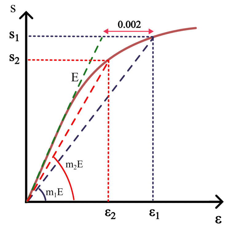
The yield strength $S_Y$ and factor $\alpha = \left( \frac{S_Y}{K’} \right)^{\frac{1}{n’}}$ are often taken at \(\varepsilon_{\text{PY}}\)=0.002 (i.e., 0.2%). In such cases, Equation 10 becomes:
$$\varepsilon_{\text{total}} = \frac{S}{E} + 0.002 \left(\frac{S}{S_Y} \right)^{\frac{1}{n’}}\tag{11}$$
This strain hardening exponent n‘ can be approximated using yield and ultimate values via the following relationship:
$$n’ = \frac{\log(S_U) – \log(S_Y)}{\log(\varepsilon_{\text{PU}}) – \log(\varepsilon_{\text{PY}})}\tag{12}$$
Where:
$S_U$ is the utlitmate strength
$S_Y$ is the yield strength
\(\varepsilon_{\text{PU}}\) is the strain at utlimates strength
\(\varepsilon_{\text{PY}}\) is the strain at yield, typically taken as 0.2%
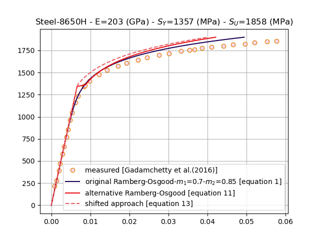
As the yield strength is taken at plastic strain of 0.2%, the alternative Ramberg-Osgood equation shows a discontinuity around the yield region. As a result, to eliminate this discontinuity the curve is shifted by 0.002 as specified in equation 13, known as shifted approach.
$$\varepsilon_{\text{total}} = \frac{S}{E} + 0.002 \left(\frac{S}{S_Y} \right)^{\frac{1}{n’}} – 0.002 \tag{13}$$
Although the shifting can cause deviation from the actual data and result in considerable error. As an example, Figure 5 compares the original, alternative and approcah methods for steel 8650H with the measured stress-strain data (Gadamchetty et al. (2016)). As seen, the removal of the discontinuity in the alternative approach causes an error in the curve predicted by the shift approach.
Thus, when only the yield and utlitmate strength points are known, the alternative Ramberg–Osgood model (Equation 11) offers a practical means to estimate the true stress–strain behavior of materials lacking full experimental data and no knowledge of work hardening exponent.
References
I am a mechanical engineer in the fields of thermal energy storage, fluid mechanics and heat transfer. I have obtained my PhD from KTH Royal Institute of Technology in designing robust and compact additively manufactured prototypes. During my PhD, I worked on CFD modeling and optimization of innovative heat exchanger designs and conducted experiments of the manufactured prototypes in laboratory environments.
In June 2019, I managed to secure the funding for continuation of my PhD by receiving a grant of 3.7 MSEK from the Swedish Energy Agency on development of 3Dprineted air-PCM heat exchangers.
