Neuber's Rule in FEA: The Complete Guide to Plasticity Correction
What Is Neuber's Rule in FEA?
Neuber’s rule is a post-processing method used in Finite Element Analysis (FEA) to convert artificially high, pseudo-elastic stress from a linear solver into a realistic elastic-plastic stress and strain estimate. By preserving the product of stress and strain ($\sigma \cdot \varepsilon = \text{constant}$), it allows engineers to accurately predict local plasticity and high-cycle fatigue life at notches without the high computational cost of running a full nonlinear FEA.
Key Takeaways
What it does: Converts pseudo-elastic stress from linear FEA into realistic elastic-plastic results without rerunning the solver.
The physics: Preserves the product of stress and strain, geometrically equating the rectangular area under the elastic solution to that of the corrected elastic-plastic solution.
Best for: Localized plasticity at stress concentrations, high-cycle fatigue life prediction, and rapid concept design screening.
Neuber vs. Glinka: Neuber preserves the stress-strain product (more conservative); Glinka preserves the Strain Energy Density (closer to experimental correlation).
Critical limitation: Only valid for small, localized plastic deformation. Widespread plasticity requires a full nonlinear analysis.
Table of Contents
The Core Problem: Why Linear FEA Overpredicts Stress
Linear elastic FEA solvers follow Hooke’s Law unconditionally. The solver has no concept of yielding. When the computed stress exceeds the material’s yield strength, the solver keeps going along that linear path and reports a fictitious value called the pseudo-elastic stress.
This is not the real stress in the structure. The actual material yields, redistributes load, and follows its nonlinear stress-strain curve. The pseudo-elastic stress can be two, three, or even five times higher than what the material physically experiences.
This matters because downstream engineering decisions depend on accurate local stress and strain. Fatigue life prediction requires the true elastic-plastic state at the critical location. Feed it pseudo-elastic stress, and your life estimates are meaningless.
You have two options to fix this:
Run a full elastic-plastic (nonlinear) analysis: Highly accurate, but costs significantly more compute time for large models with many load cases.
Apply a plasticity correction: A fast post-processing operation on linear results. Neuber’s rule is the industry standard for this correction.
What Is Neuber's Rule? A Clear Definition
Neuber’s rule estimates the real elastic-plastic stress and strain at a stress concentration from linear FEA results. It does this by preserving the product of stress and strain during the correction from the elastic to the elastic-plastic domain.
Formulated by Heinz Neuber in 1961, he proposed that the theoretical stress concentration factor ($K_t$) equals the geometric mean of the actual stress concentration factor ($K_\sigma$) and the actual strain concentration factor ($K_\varepsilon$):
The Neuber Formula Explained
The governing equation of Neuber’s rule for FEA applications is:
Where:
$\sigma^e$ = pseudo-elastic stress from linear FEA (the value exceeding yield)
$\varepsilon^e$ = elastic strain from FEA, equal to $\sigma^e / E$
$\sigma^N$ = Neuber-corrected elastic-plastic stress
$\varepsilon^N$ = Neuber-corrected elastic-plastic strain
$E$ = Young’s modulus
Geometric Interpretation
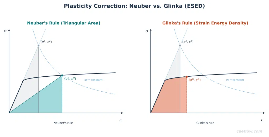
On a stress-strain diagram, the elastic solution sits on the linear elastic line, above the yield point. Neuber’s rule defines a constant-product hyperbola passing through this point. The corrected elastic-plastic solution lies at the intersection of this hyperbola and the material’s actual stress-strain curve.
The geometric meaning is that the rectangular area formed by the elastic solution equals the rectangular area formed by the corrected solution on the real curve. The stress goes down, the strain goes up, and the product stays constant.
Neuber vs. Glinka: Which Plasticity Correction Should You Use?
Most fatigue solvers offer two plasticity correction methods: Neuber and Glinka (Equivalent Strain Energy Density, or ESED). Both start from the same linear input but preserve different physical quantities.
Neuber’s Rule: Preserves the stress-strain product (the rectangular area).
Glinka’s Rule (ESED): Preserves the strain energy density (the area under the stress-strain curve):
| Feature | Neuber Method | Glinka (ESED) Method |
|---|---|---|
| Physical Principle | Equates the Rectangular Area (stress-strain product) to the material's energy state. | Equates the Actual Strain Energy Density (area under the curve) to the elastic energy. |
| Governing Equation | σ · ε = Constant | ∫ σ dε = Elastic Strain Energy |
| Bias | Conservative (Predicts higher strain, typically safer) |
Less Conservative (Predicts lower strain, closer to mean) |
| Best Application | General fatigue design & safety-critical parts | Correlation with experimental data or high-accuracy optimization |
The Verdict: For most durability and fatigue design work, use Neuber. It is the industry default. Use Glinka when correlating with test data or when Neuber causes severe overdesign.
Try it yourself: Use the interactive calculator below to see exactly how Neuber and Glinka corrections compare across different materials and pseudo-elastic stress levels.
Interactive Notch Plasticity Correction
Step-by-Step Workflow: Calculating Neuber Stress
Follow this procedure to convert your FEA results manually or via scripts.
Step 1: Run Linear Elastic FEA
Set up your model with linear elastic material properties. Run the analysis and extract the peak pseudo-elastic stress ($\sigma^e$) at the critical location. Ensure your mesh is refined at the hotspot; Neuber cannot fix a poorly converged linear stress.
Step 2: Define the Neuber Constant
Compute the stress-strain product from your elastic results to define the Neuber hyperbola:
Step 3: Select the Material Model
You need the material’s nonlinear response. For fatigue, use the stabilized cyclic stress-strain curve. You can represent this in two ways:
Ramberg-Osgood equation: Uses the cyclic strength coefficient ($K’$) and cyclic strain hardening exponent ($n’$).
Tabular data: A direct set of yield stress vs. plastic strain data points, used for irregular hardening behavior.
Step 4: Solve the System
Substitute the material curve into the Neuber equation:
For the Ramberg-Osgood form, this becomes a single nonlinear equation solved iteratively:
To know more about Ramberg-Osgood, please read our blog : ramberg-osgood-stress-strain
When to Use Neuber's Rule (and When Not To)
Use It When
Plasticity is highly localized — confined to a notch root, hole edge, fillet, or weld toe, while the surrounding material remains elastic. This is the fundamental assumption.
You are performing fatigue or durability analysis — most commercial fatigue solvers (fe-safe, nCode DesignLife, FEMFAT, CAEfatigue) rely on Neuber-type corrections as part of their standard strain-life workflow.
You are screening multiple concept designs — running hundreds of load cases through full nonlinear analyses is impractical during early design. Linear elastic + Neuber gives a physically grounded screening metric at a fraction of the cost.
Loading is proportional and monotonic — or you are extending to cyclic loading using the Masing hypothesis with the cyclic stress-strain curve scaled by a factor of two.
Do NOT Use It When
Plasticity is widespread — if yielding extends over a large portion of the cross-section, the elastic stress distribution is too far from reality for a local correction to recover. The global load path is wrong. You need a full nonlinear analysis.
You need accurate displacements or reaction forces — Neuber’s rule is output-only. It corrects stress and strain at a point. It does not alter the stiffness matrix, equilibrium, or displacement field.
Geometric nonlinearity is significant — large deformations combined with plasticity require a nonlinear solver.
The material is anisotropic or non-metallic — Neuber’s rule assumes isotropic, rate-independent plasticity with a smooth stress-strain curve.
Rule of Thumb
If the peak stress is less than roughly 2–3× the yield strength and the yielding is confined to a small volume near a stress raiser, Neuber’s rule is a reasonable approximation. Beyond that range, the assumptions degrade and you should invest in a nonlinear solve.
Summary
Neuber’s rule is a foundational method in the structural analyst’s toolkit. It bridges the gap between the computational efficiency of linear elastic FEA and the physical accuracy of nonlinear plasticity — as long as you respect its core assumption: plasticity must be small and localized.
Use it to convert pseudo-elastic stress into realistic elastic-plastic estimates for fatigue, durability, and concept design workflows. Pair it with a proper cyclic material model, and you get physically meaningful results at a fraction of the nonlinear solve cost.
It is not a replacement for full nonlinear analysis. It is a proven, efficient shortcut for the right class of problems.
Finally, if you’d like to know more about FEA automation or CAE in general, please visit CAEFLOW or follow us on social media:
Frequently Asked Questions (FAQ)
What is Neuber’s rule in simple terms?
Neuber’s rule is a calculation method that takes the artificially high stress from a linear FEA model and scales it down to a realistic elastic-plastic value by finding where a constant-energy hyperbola intersects the material’s real stress-strain curve.
What is the difference between Neuber and Glinka correction?
Neuber preserves the rectangular area on the stress-strain diagram (stress times strain). Glinka preserves the actual area under the curve (strain energy density). Neuber is generally more conservative and predicts a shorter fatigue life.
Does Neuber’s rule change the FEA solution?
No. It is purely a post-processing step. It does not modify the solver’s stiffness matrix, equilibrium solution, or displacement results.
Is Neuber’s rule conservative?
Yes, especially relative to Glinka and full nonlinear analysis. It tends to slightly overpredict local strain, making it a safer, more conservative choice for engineering design.
What is the Neuber constant?
The Neuber constant is the fixed product of linear stress and linear strain at your critical node. It defines the exact hyperbola curve that must be matched by your corrected elastic-plastic solution.
References (clickable):
- Neuber, H., “Theory of Stress Concentration for Shear-Strained Prismatical Bodies with Arbitrary Nonlinear Stress-Strain Law,” Journal of Applied Mechanics, vol. 28, pp. 544–550, 1961.
- Molski, K., and G. Glinka, “A Method of Elastic-Plastic Stress and Strain Calculation at a Notch Root,” Materials Science and Engineering, vol. 50, pp. 93–100, 1981.
- How to Model True Stress–Strain Curves with missing strain hardening coefficient for plastic deformations

I am a senior CAE and Automation Engineer at Scania with over 8 years of hands-on experience in Finite Element Analysis (FEA). My daily work involves advanced simulations focusing on strength and durability analysis, helping design more reliable and efficient products.
Before joining Scania, I conducted research at KTH Royal Institute of Technology, where I focused on the additive manufacturing of heat exchangers. My work has been recognized internationally and published in peer-reviewed journals. You can find my publications on Google Scholar.
In June 2019, I managed to secure the funding for continuation of my PhD by receiving a grant of 3.7 MSEK from the Swedish Energy Agency on development of 3Dprineted air-PCM heat exchangers.