Static General
Nonlinear geometry, material nonlinearity, contact, and large deformations.
Choosing the wrong analysis type in Abaqus is one of the most expensive mistakes you can make in finite element analysis — and I’ve seen it happen more times than I’d like to admit.
You set up your model, define your boundary conditions, run the simulation overnight, come back in the morning, and realize you used Dynamic Explicit when you should have used Static General. Hours wasted. Or worse, you get results that look reasonable but are completely wrong because you didn’t account for the actual physics of your problem.
Abaqus, developed by Dassault Systèmes under the SIMULIA brand, is one of the most powerful FEA software packages available. It provides two main solvers — Abaqus/Standard for implicit analysis and Abaqus/Explicit for explicit dynamics — along with Abaqus/CFD for computational fluid dynamics. Together, these solvers offer over 25 different analysis procedures based on the finite element method.
This FEA analysis guide exists because I got tired of digging through documentation every time I needed to remember the difference between SSD Modal and SSD Direct, or when exactly I should switch from implicit to explicit dynamics. Whether you’re learning FEA or need a quick reference, this FEA analysis guide has you covered.
This FEA analysis guide covers all 28+ Abaqus procedures with practical recommendations for each.
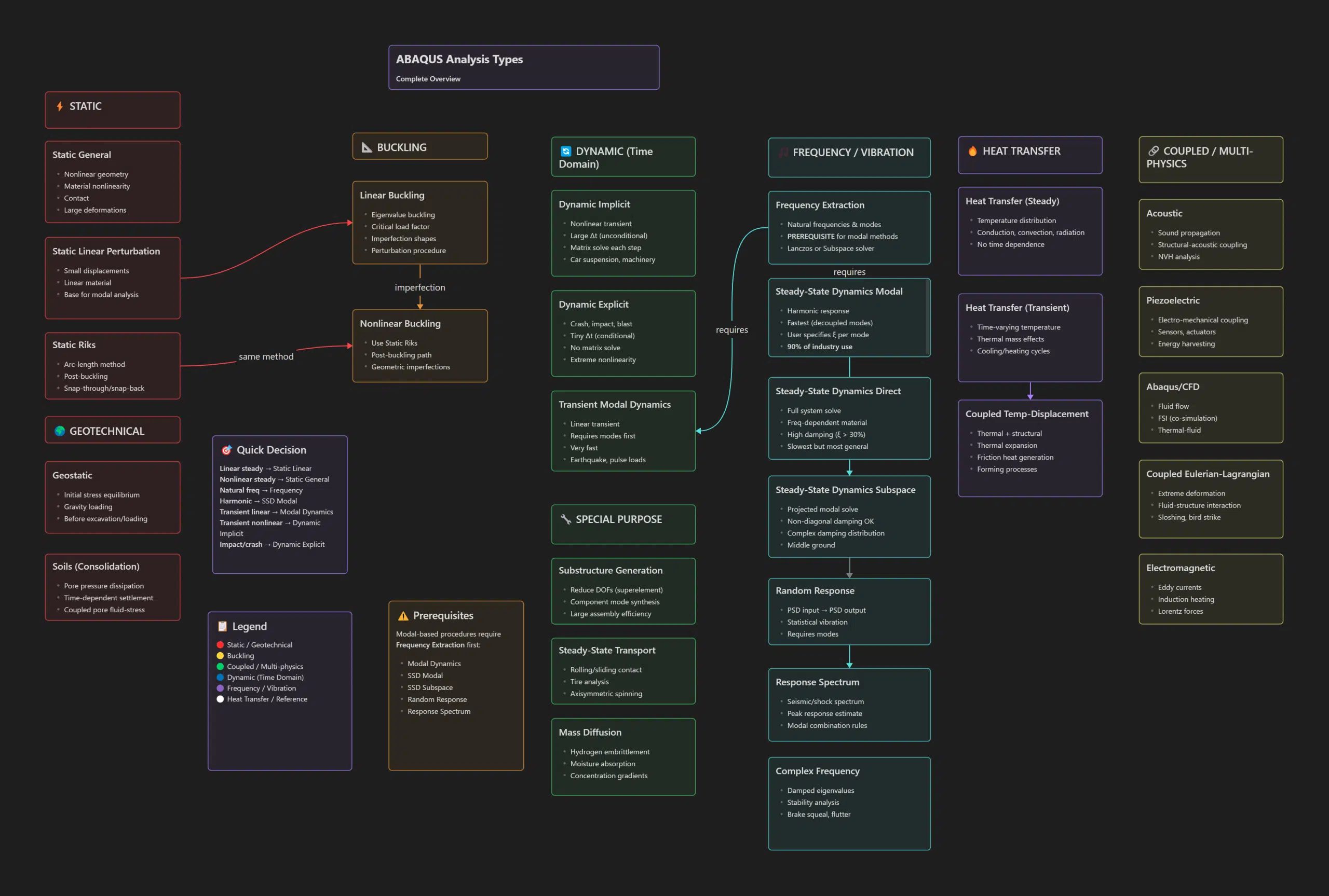
Abaqus analysis types are the different simulation procedures available in Abaqus FEA software for solving structural, thermal, and multi-physics problems. Each analysis type uses a specific mathematical approach to solve the governing differential equations, and selecting the right one depends on your loading conditions, material behavior, and the physics you need to capture.
The 8 main Abaqus analysis categories are:
The interactive FEA analysis guide below lets you filter by category and find the exact procedure you need.
Complete visual reference for all FEA analysis procedures in Abaqus/Standard, Abaqus/Explicit, and Abaqus/CFD.
Nonlinear geometry, material nonlinearity, contact, and large deformations.
Small displacements, linear material. Base for modal analysis.
Arc-length method for snap-through and snap-back instabilities.
Eigenvalue buckling for critical load factors and imperfection shapes.
Uses Static Riks with geometric imperfections for post-buckling path.
Nonlinear transient with unconditionally stable time stepping. Matrix solve each step.
Extreme nonlinearity with conditionally stable tiny time steps. No matrix solve.
Linear transient using modal superposition. Very fast.
Natural frequencies and mode shapes. Required for all modal-based methods.
Harmonic response with decoupled modes. User specifies ξ per mode.
Projected modal solve. Non-diagonal damping OK. Middle ground approach.
Full system solve for frequency-dependent materials and high damping. Slowest but most general.
PSD input → PSD output. Statistical vibration analysis. Requires modes.
Seismic/shock spectrum with modal combination rules for peak response estimate.
Damped eigenvalues for stability analysis.
Temperature distribution via conduction, convection, radiation. No time dependence.
Time-varying temperature with thermal mass effects. Cooling/heating cycles.
Combined thermal and structural. Thermal expansion, friction heat generation.
Sound propagation and structural-acoustic coupling for NVH analysis.
Electro-mechanical coupling for sensors, actuators, energy harvesting.
Fluid flow with FSI co-simulation and thermal-fluid coupling.
Extreme deformation problems with fluid-structure interaction.
Eddy currents, induction heating, and Lorentz forces.
Reduce DOFs via component mode synthesis for large assembly efficiency.
Rolling/sliding contact analysis. Tire analysis, axisymmetric spinning.
Concentration gradients for hydrogen embrittlement and moisture absorption.
Initial stress equilibrium under gravity. Run before excavation/loading.
Pore pressure dissipation, time-dependent settlement, coupled pore fluid-stress.
These procedures require Frequency Extraction first:
Workflow Tip:
Always run frequency extraction first when planning modal-based analyses. The extracted modes become the basis for efficient dynamic solutions.
The finite element method gives you tremendous power to simulate structural behavior — but that power requires choosing the right analysis procedure for your problem physics. This FEA analysis guide covered the 8 main categories and 28+ procedures available in Abaqus. Bookmark this finite element analysis guide for quick reference during your simulation work.. For more on automating repetitive FEA tasks once you’ve mastered analysis selection, see our guide on FEA automation and Sine Sweep.
Abaqus/Standard uses implicit time integration with large time steps and requires matrix solving at each increment — ideal for static and low-speed dynamic problems. Abaqus/Explicit uses explicit integration with very small time steps and no matrix inversion — best for high-speed impacts, crash simulations, and extreme nonlinearity.
Use Dynamic Explicit for crash, impact, blast, and problems with extreme nonlinearity where events happen in milliseconds. Use Dynamic Implicit for slower transient events like machinery vibration or car suspension dynamics where larger time steps are acceptable and computational stability is preferred.
Frequency Extraction is an Abaqus analysis procedure that calculates the natural frequencies and mode shapes of a structure. It uses eigenvalue solvers (Lanczos or Subspace) and is a required prerequisite for all modal-based dynamic analyses including Modal Dynamics, Steady-State Dynamics, Random Response, and Response Spectrum.
SSD Modal (Steady-State Dynamics Modal) is a harmonic response analysis in Abaqus that calculates how a structure responds to sinusoidal loading at various frequencies. It uses pre-computed mode shapes from Frequency Extraction and is the fastest harmonic analysis method, used in approximately 90% of industry NVH applications.
Choose your FEA analysis type based on: (1) loading type — static or time-varying, (2) material behavior — linear or nonlinear, (3) deformation magnitude — small or large, (4) time scale — quasi-static, transient, or impact. For most problems, start with Static General. For vibration, use Frequency Extraction followed by the appropriate dynamic procedure.

I am a senior CAE and Automation Engineer at Scania with over 8 years of hands-on experience in Finite Element Analysis (FEA). My daily work involves advanced simulations focusing on strength and durability analysis, helping design more reliable and efficient products.
Before joining Scania, I conducted research at KTH Royal Institute of Technology, where I focused on the additive manufacturing of heat exchangers. My work has been recognized internationally and published in peer-reviewed journals. You can find my publications on Google Scholar.
In June 2019, I managed to secure the funding for continuation of my PhD by receiving a grant of 3.7 MSEK from the Swedish Energy Agency on development of 3Dprineted air-PCM heat exchangers.