y+ Calculator and Wall Treatment in CFD: Wall Functions and First Cell Height
Key Takeaways
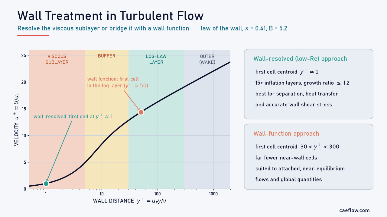
- Wall treatment decides how a CFD model handles the thin layer next to a wall, where the velocity drops to zero and viscosity takes over from turbulence. You either resolve the viscous sublayer with fine cells (first cell at $y^+ \approx 1$) or bridge it with a wall function (first cell at roughly $30 < y^+ < 300$).
- y+ is the wall distance in viscous units, $y^+ = u_\tau y/\nu$. It tells you which layer of the boundary layer the first cell centre sits in, and it can only be confirmed once the solution exists.
- Standard wall functions assume an attached boundary layer in equilibrium. In a backward-facing-step benchmark they predicted a reattachment length 28% too short, while a pressure-gradient-sensitive wall function and a low-Re model were 6–7% short (Shih et al., 2003).
- Keep the first cell out of the buffer layer ($5 < y^+ < 30$) unless your wall treatment is designed to be y+-insensitive.
- The first-cell height follows from a skin-friction estimate: for air at 30 m/s over a 2 m car roof, $y^+ = 1$ puts the first cell centre about 13 µm from the wall (a 26 µm cell), while $y^+ = 50$ allows about 0.65 mm.
Table of Contents
- Key Takeaways
- Introduction
- What Is Wall Treatment in CFD?
- The Turbulent Boundary Layer and the Viscous Sublayer
- The Law of the Wall
- Wall Functions: Bridging the Viscous Sublayer
- Resolving the Viscous Sublayer
- Wall Treatment by Turbulent Flow Type
- Choosing y+ and the First-Cell Height
- Worked Example
- Strengths and Limitations
- Conclusion
- Interactive y+ Calculator
- FAQ
- References
Introduction
Almost every engineering flow touches a wall: air over a car roof, water in a pipe, hot gas through a turbine passage. Next to the wall the velocity falls to zero within a fraction of a millimetre, and viscosity takes over from turbulence. How a CFD model handles this thin region is called wall treatment, and it often controls the predicted drag, pressure drop, heat transfer and separation point as much as the turbulence model itself.
The difficulty is scale. Resolving the near-wall gradients needs cells only micrometres thick, which multiplies the cell count and, in unsteady runs, shrinks the time step. Wall functions avoid this with an empirical law, but that law was derived for attached boundary layers and becomes unreliable near separation, stagnation points and strong pressure gradients.
This guide covers the viscous sublayer, the law of the wall and y+, the main wall-function and wall-resolved approaches, and the wall treatment that suits each type of turbulent flow, ending with a worked example and an interactive y+ calculator.
What Is Wall Treatment in CFD?
Wall treatment is the set of boundary conditions and model modifications that a turbulence model uses in the cells next to a solid wall. It fixes how the wall shear stress, heat flux and turbulence quantities are obtained in the viscosity-affected layer, either by resolving that layer with a fine mesh or by bridging it with semi-empirical wall functions.
Why Walls Make Turbulent Flow Hard to Model
Two-equation models such as the standard k-ε model were built for fully turbulent flow at high Reynolds number, where turbulent mixing dwarfs molecular viscosity. Near a wall that assumption fails: the no-slip condition forces the velocity to zero, the wall damps the fluctuations, and in the thinnest layer viscosity carries almost all of the shear stress. The steepest gradients are found here, and turbulence production peaks just above it.
So the model needs damping terms or a different near-wall formulation, and the mesh must either capture the steep profiles or the solver must be told their shape.
Two Strategies: Resolve the Wall or Model It
The wall-resolved (low-Reynolds-number) approach integrates the equations all the way to the wall. The first cell centre lies inside the viscous sublayer, ideally at $y^+ \approx 1$, and the turbulence model includes near-wall terms. It is the more accurate option, but it needs many thin cells.
The wall-modelled approach places the first cell centre in the logarithmic layer, roughly $30 < y^+ < 300$, and lets a wall function supply the wall shear stress and the turbulence values in that cell. In Guerrero's lecture examples, changing only the inflation layers from wall-modelling (average $y^+ \approx 60$) to wall-resolving ($y^+ \approx 1$) raised the cell count by a factor of 1.7 to 1.9 for three different geometries.
The Turbulent Boundary Layer and the Viscous Sublayer
On a smooth flat plate the boundary layer starts laminar. Downstream, small disturbances grow and the flow passes through a transition region into a turbulent boundary layer, which is thicker, fuller and far better mixed (Figure 1). For a flat plate the critical Reynolds number $\mathrm{Re}_x = \rho U_\infty x/\mu$ is often taken as about $5\times10^5$, but the actual value depends on free-stream turbulence, surface roughness and pressure gradient.
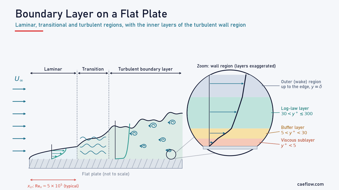
Figure 1. Development of the boundary layer on a smooth flat plate, from laminar through transition to turbulent, with a zoom of the turbulent wall region: viscous sublayer ($y^+ < 5$), buffer layer ($5 < y^+ < 30$), log-law layer and outer region. Schematic; the layer thicknesses are exaggerated.
Inside a turbulent boundary layer there is a clear separation of scales. The outer part is governed by the boundary-layer thickness $\delta$ and the free stream, while the inner part depends only on the wall shear stress and the viscosity. That is why the near-wall flow looks so similar in pipes, channels and boundary layers once it is expressed in the right units.
Wall Units: Friction Velocity, y+ and u+
Near the wall, the quantities that matter are the wall shear stress $\tau_w$, the density $\rho$ and the kinematic viscosity $\nu = \mu/\rho$. Together they define a velocity scale, the friction velocity, and from it a dimensionless wall distance and velocity:
$$u_\tau = \sqrt{\frac{\tau_w}{\rho}}, \qquad y^+ = \frac{u_\tau\,y}{\nu}, \qquad u^+ = \frac{U}{u_\tau}$$
Here $y$ is the normal distance from the wall and $U$ the mean velocity parallel to it. $y^+$ is a local Reynolds number: it compares the wall distance with the viscous length $\nu/u_\tau$, which is of the order of micrometres to tens of micrometres in typical air and water flows. Because $\tau_w$ comes out of the solution, $y^+$ can only be estimated before a run and must be checked afterwards.
The Layers Near the Wall
In wall units the inner region splits into layers whose usual limits, following Pope (2000), are:
- Viscous sublayer, $y^+ < 5$: viscous stress dominates, the flow is effectively laminar and $u^+ \approx y^+$.
- Buffer layer, $5 < y^+ < 30$: viscous and turbulent stresses are of similar size, and turbulence production peaks here.
- Log-law layer, $y^+ > 30$ and $y/\delta < 0.3$: turbulent stress dominates and the velocity varies with the logarithm of the wall distance.
- Outer (wake) region: the profile departs from the log law and depends on the pressure gradient and the free stream.
These limits are conventions rather than sharp boundaries. The upper end of the log layer, in wall units, grows with Reynolds number; at low Reynolds number the log layer is short and a wall function has little room to work.
The Law of the Wall
The law of the wall describes the mean velocity in the inner layers. In the viscous sublayer the shear stress is nearly constant and purely viscous, which gives a linear profile. In the log layer, dimensional reasoning and measurements give a logarithmic one:
$$\begin{gathered} u^+ = y^+ \quad (y^+ \lesssim 5) \\ u^+ = \frac{1}{\kappa}\ln y^+ + B \quad (y^+ \gtrsim 30) \end{gathered}$$
$\kappa \approx 0.41$ is the von Kármán constant and $B$ lies between about 5.0 and 5.5 depending on the source; we use $B = 5.2$ (Pope, 2000). Ansys Fluent writes the log law as $U^* = \ln(E\,y^*)/\kappa$ with $\kappa = 0.4187$ and $E = 9.793$, which corresponds to $B \approx 5.45$.
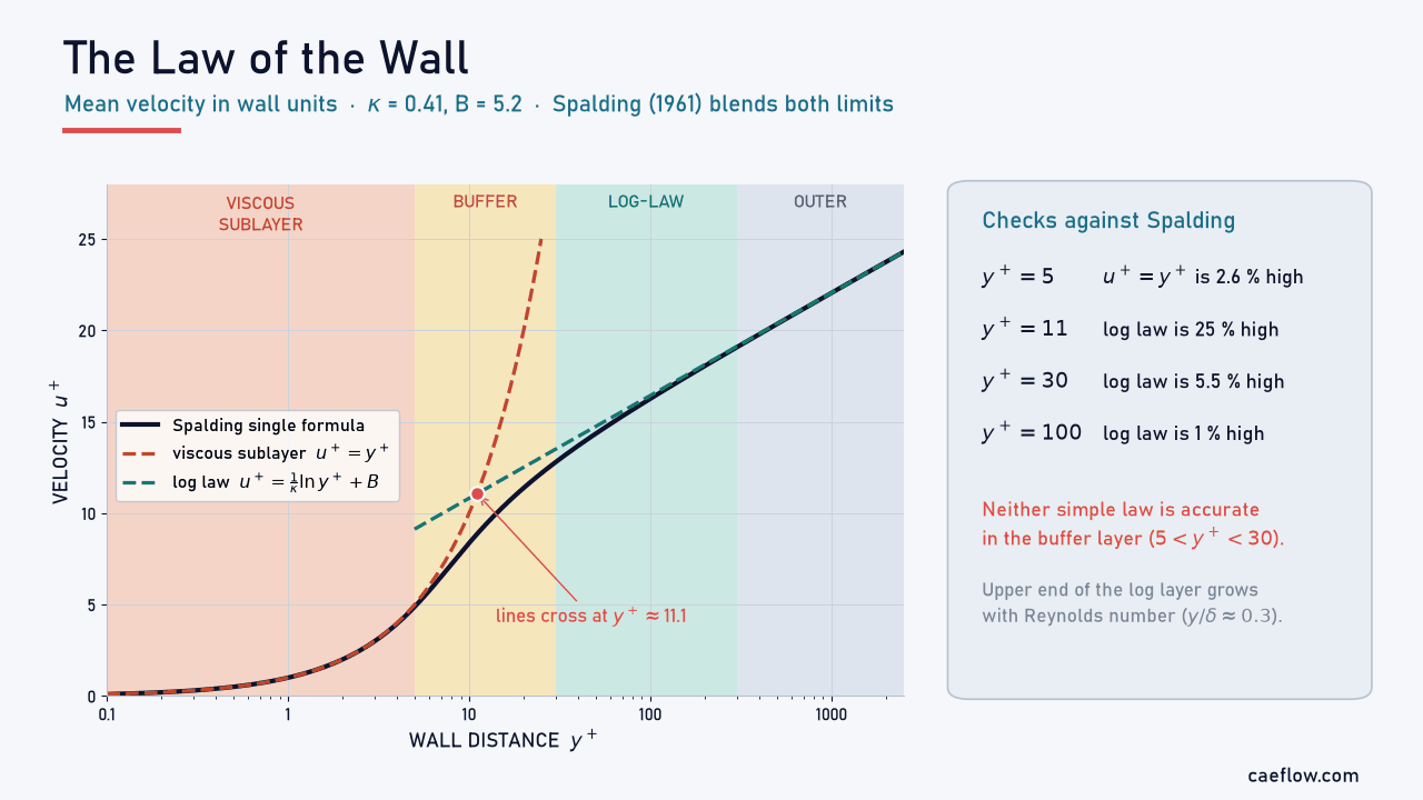
Figure 2. Law of the wall with $\kappa = 0.41$ and $B = 5.2$. The linear sublayer law and the log law cross at $y^+ \approx 11.1$, and Spalding's single formula follows both limits and the buffer layer between them. Compared with Spalding, the log law is 25% high at $y^+ = 11$ and 5.5% high at $y^+ = 30$.
The two simple laws cross at $y^+ \approx 11$ (11.06 with our constants, 11.225 with Fluent's). Neither is accurate in the buffer layer, which is why practical wall treatments either keep the first cell out of it or use a blended profile. Spalding (1961) proposed a single formula that holds from the wall through the log layer:
$$\begin{aligned} y^+ = u^+ + e^{-\kappa B}\Big[ & e^{\kappa u^+} - 1 - \kappa u^+ \\ & - \frac{(\kappa u^+)^2}{2} - \frac{(\kappa u^+)^3}{6} \Big] \end{aligned}$$
Blended profiles of this kind, and Kader's (1981) blending for velocity and temperature, are the basis of the y+-insensitive wall treatments described below.
Wall Functions: Bridging the Viscous Sublayer
A wall function is a set of formulas that links the solution in the first cell to the wall, so that the viscous sublayer and the buffer layer never need to be meshed. From the velocity at the first cell centre it returns the wall shear stress, and it also sets the turbulence quantities in that cell.
Standard Wall Functions (Launder–Spalding)
The classic formulation of Launder and Spalding (1974), still the default in many codes, does not use $u_\tau$ directly. It builds the velocity scale from the turbulent kinetic energy $k_P$ at the first cell centre P:
$$\begin{gathered} y^* = \frac{\rho\,C_\mu^{1/4}k_P^{1/2}\,y_P}{\mu} \\ U^* = \frac{U_P\,C_\mu^{1/4}k_P^{1/2}}{\tau_w/\rho} = \frac{1}{\kappa}\ln\left(E\,y^*\right) \end{gathered}$$
With $C_\mu = 0.09$, this returns $\tau_w$ from $U_P$, $k_P$ and $y_P$. Using $k$ instead of $u_\tau$ avoids a singularity where the wall shear stress vanishes. In local equilibrium, where turbulence production balances dissipation, $y^*$ equals $y^+$; the dissipation rate in the wall cell is also set from this assumption rather than solved.
The formulation has two weaknesses. It assumes an equilibrium log layer, and it degrades under mesh refinement: Ansys notes that, for all but scalable wall functions, $y^+$ values below about 15 gradually cause unbounded errors in wall shear stress and heat transfer. A finer mesh can give a worse answer.
Scalable Wall Functions
Scalable wall functions remove the refinement problem by limiting the wall distance used in the formula, $\tilde{y}^* = \max(y^*, 11.225)$ in Fluent. If the first cell falls into the viscous sublayer, the solver treats it as if it sat at the edge of the log layer. Results become consistent under refinement, but the sublayer is still not resolved, so the accuracy remains that of a wall function.
Non-Equilibrium and Generalized Wall Functions
Pressure gradients bend the near-wall profile away from the standard log law: an adverse gradient decelerates the flow, as in a diffuser, and a favourable one accelerates it, as in a nozzle. Non-equilibrium wall functions (Kim & Choudhury, 1995) make the log law sensitive to the pressure gradient. Ansys recommends them for separation, reattachment and impingement, but warns that they lose reliability for severe pressure gradients, strong body forces and highly three-dimensional near-wall flow.
The generalized wall function of Shih, Povinelli and Liu (2003) adds a pressure-gradient velocity scale, $u_p = \left(\nu\,|dP_w/dx|/\rho\right)^{1/3}$, to $u_\tau$. It reduces to the log law at zero pressure gradient and to a pressure-gradient law at zero wall shear stress, and it is fitted across all three inner layers, so the first cell can sit anywhere in them.
Defect Wall Functions in High-Speed Flow
Wall functions also work at high speed. In a NASA study, Brown (1994) added the Barnwell–Wahls defect wall function to a Parabolized Navier–Stokes code for supersonic flat plates. The wall shear stress came analytically from the laws of the wall and the wake and a defect-stream function, with a matching slip velocity imposed at the wall.
Against fully gridded solutions with the first point at $y^+ \le 1$–2, run time fell by factors of about 30, 9 and 5 at Mach 2, 5 and 8. The price was accuracy: at the trailing edge the wall shear stress differed by about 15% at Mach 2 and by 25% and 40% at Mach 5 and 8.
Resolving the Viscous Sublayer: Low-Re and y+-Insensitive Wall Treatment
When wall shear stress, heat transfer or the separation point matter, the safer route is to resolve the viscous sublayer. Low-Reynolds-number turbulence models add damping functions or near-wall terms so that $k$, the eddy viscosity and the dissipation behave correctly as $y \to 0$. The mesh must then place the first cell centre at about $y^+ = 1$ and grow gently away from the wall (Figure 3).
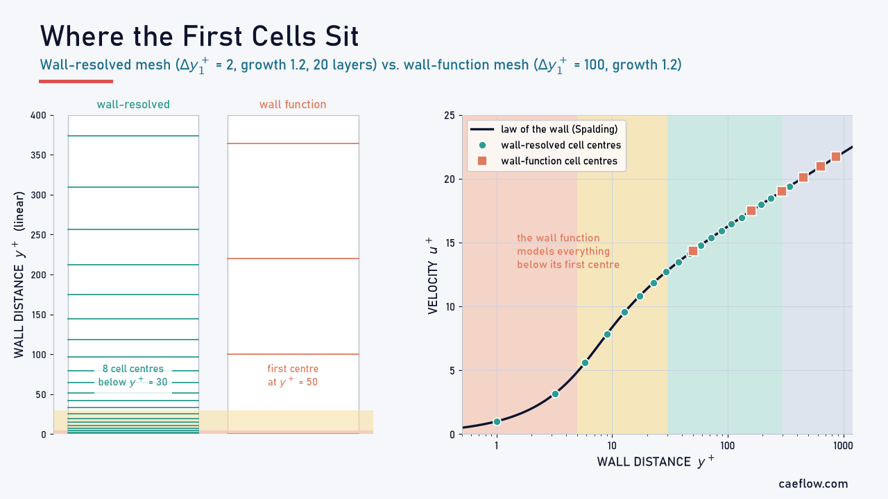
Figure 3. Cell centres of a wall-resolved mesh (first-cell height $\Delta y_1^+ = 2$, growth ratio 1.2, 20 layers) and a wall-function mesh ($\Delta y_1^+ = 100$, growth ratio 1.2) on the law of the wall. The wall-resolved mesh puts 8 cell centres below $y^+ = 30$; the wall-function mesh puts none, and its first centre sits at $y^+ = 50$.
Two-Layer Models and Enhanced Wall Treatment
For ε-based models, a practical alternative is the two-layer approach of Wolfshtein (1969), summarised clearly in Bakker's CFD lecture notes. The domain is split with a wall-distance Reynolds number, $\mathrm{Re}_y = \rho\,y\sqrt{k}/\mu$. Where $\mathrm{Re}_y$ is below a threshold (200 in Fluent), only the $k$ equation is solved, and $\varepsilon$ and the eddy viscosity come from algebraic length scales; further out, the full k-ε model applies. Fluent's Enhanced Wall Treatment combines this with blended wall laws, so it works on fine meshes and degrades gracefully on coarse ones.
k-ω SST and y+-Insensitive Wall Treatment
The k-ω family, including Menter's (1994) SST model, can be integrated to the wall without damping functions, because $\omega$ has a known analytical behaviour next to the wall. Current implementations blend the viscous-sublayer and log-law forms of $\omega$ and the wall shear stress, which makes them y+-insensitive: they give consistent results whether the first cell sits at $y^+ \approx 1$ or in the log layer. The Spalart–Allmaras model and Fluent's Menter–Lechner ε formulation follow the same idea.
Insensitive does not mean equally accurate everywhere. Guerrero recommends aiming for $y^+$ of 1 to 2 on resolved meshes (values up to 6 or 7 cost little accuracy) with at least 15 inflation layers at a growth ratio of 1.2 or less. Pushing below $y^+ = 0.1$ brings little benefit and can spoil cell quality.
Wall Treatment by Turbulent Flow Type
The right wall treatment depends less on the software than on how far the near-wall flow departs from the equilibrium boundary layer that wall functions assume. Figure 4 groups common turbulent flows into four types.
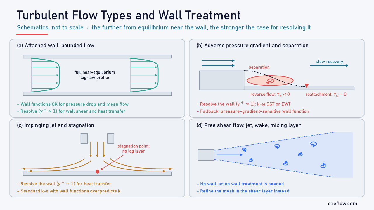
Figure 4. Four types of turbulent flow and the wall treatment that suits each: (a) attached wall-bounded flow, (b) adverse pressure gradient and separation, (c) impinging jet with a stagnation point, (d) free shear flow away from walls. Schematics, not to scale.
Free Shear Flows: Jets, Wakes and Mixing Layers
In a free jet, a wake or a mixing layer, turbulence is produced by velocity differences inside the fluid rather than by a wall. Wall treatment hardly matters here; resolving the shear layers does. Walls enter the problem only where the jet or wake meets a surface, and the flow there becomes one of the types below.
Attached Wall-Bounded Flows
Fully developed pipe and duct flow, flat plates and attached boundary layers with mild pressure gradients are the home ground of the law of the wall. Standard or scalable wall functions give good pressure drop and mean velocity with far fewer cells, and Shih et al. (2003) reproduced flat-plate skin friction and velocity profiles with grids of 5 to 100 points across the boundary layer using their generalized wall function.
Recommended treatment: wall functions with the first cell at $30 < y^+ < 300$ for pressure drop and mean flow; a wall-resolved mesh at $y^+ \approx 1$ when skin friction or heat transfer is the result you need.
Flows with Pressure Gradients
Diffusers, nozzles, turbomachinery blades and airfoils at high lift impose streamwise pressure gradients. An adverse gradient thickens the boundary layer and pulls the near-wall velocity away from the standard log law, and a favourable one pushes it the other way. Standard wall functions ignore the gradient, so their wall shear stress error grows with it.
Recommended treatment: a wall-resolved mesh with k-ω SST or Enhanced Wall Treatment; if the mesh must stay coarse, a pressure-gradient-sensitive (non-equilibrium or generalized) wall function.
Separated and Reattaching Flows
Separation is where the assumptions behind standard wall functions break down completely. At the separation and reattachment points $\tau_w = 0$, so $u_\tau = 0$ and $y^+$ loses its meaning; inside the recirculation bubble the wall shear stress reverses sign (Figure 5). The near-wall flow is far from equilibrium, and the log law does not hold there.

Figure 5. Backward-facing step: separation at the step edge, recirculation with reversed wall shear stress, and reattachment at $x_R$. Reattachment lengths computed by Shih et al. (2003) on one grid for the Kim, Kline and Johnston experiment ($x_R/h = 7.0 \pm 0.5$): standard wall function 5.05 (−28%), generalized wall function 6.56 (−6%), low-Re k-ε 6.54 (−7%).
The backward-facing step puts numbers on this. On one grid, a standard wall function predicted a reattachment length $x_R/h$ of 5.05 against a measured $7.0 \pm 0.5$, 28% too short, while the generalized wall function (6.56) and a low-Re k-ε model (6.54) fell inside the experimental range. Because the three runs shared one grid, part of the standard wall function's error may come from first cells below the log layer.
The NASA Turbulence Modeling Resource uses the related Driver and Seegmiller step ($x_R/H = 6.26 \pm 0.10$) as a standard validation case.
Recommended treatment: resolve the viscous sublayer ($y^+ \approx 1$) with k-ω SST or a comparable low-Re model, and treat standard wall-function results near separation as qualitative.
Impinging Jets and Stagnation Flows
Jet-impingement cooling, the leading edge of a blade and the front of a bluff body all have a stagnation point, where the flow meets the wall head-on. There is no log layer at that point, and two-equation models such as standard k-ε overpredict the turbulent kinetic energy under strong normal strain, the stagnation-point anomaly described by Durbin (1996). The result is inflated heat transfer, and a wall function adds its own error on top.
Recommended treatment: a wall-resolved mesh ($y^+ \approx 1$) with a model or option that limits stagnation-point production of $k$; non-equilibrium wall functions only when a coarse mesh is unavoidable.
Heat Transfer, Transition and Unsteady Flows
Wall heat flux depends on the thermal sublayer just as wall shear stress depends on the viscous sublayer, so heat transfer studies generally need a resolved wall. Transition models are stricter still: Ansys states that Transition SST needs $y^+ \approx 1$, and that above about 5 the predicted transition onset moves upstream as $y^+$ grows.
In large eddy simulation the cost argument is stronger. Choi and Moin (2012) estimated that grid points for wall-resolved LES of a boundary layer grow as $\mathrm{Re}_{L_x}^{13/7}$, but only as $\mathrm{Re}_{L_x}$ for wall-modelled LES.
Choosing y+ and the First-Cell Height
Because $\tau_w$ is unknown before the run, the first-cell height is estimated from a skin-friction correlation. For a smooth flat plate of length $L$:
$$\begin{gathered} \mathrm{Re}_L = \frac{\rho U_\infty L}{\mu} \\ c_f = \left[2\log_{10}\mathrm{Re}_L - 0.65\right]^{-2.3} \\ \tau_w = \tfrac{1}{2}\,c_f\,\rho\,U_\infty^2 \end{gathered}$$
This is Schlichting's local skin-friction correlation for a smooth turbulent flat plate, valid up to $\mathrm{Re}_x \approx 10^9$. With $\tau_w$ known, the friction velocity follows, and so does the wall distance for a target $y^+$:
$$u_\tau = \sqrt{\tau_w/\rho}, \qquad y_P = \frac{y^+\,\mu}{\rho\,u_\tau}, \qquad \Delta y_1 = 2\,y_P$$
The factor of two matters. Cell-centred finite-volume codes such as Fluent evaluate $y^+$ at the centroid of the wall cell, a distance $y_P$ from the wall, so the first-cell height to enter in the mesher is $\Delta y_1 = 2y_P$. Vertex-centred codes measure the distance to the first node off the wall, so there the first-cell height equals that distance.
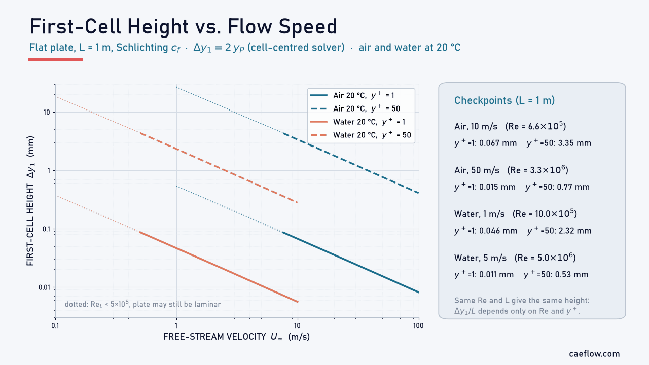
Figure 6. First-cell height $\Delta y_1 = 2y_P$ against free-stream velocity for air and water at 20 °C on a 1 m flat plate (Schlichting $c_f$), for $y^+ = 1$ and $y^+ = 50$. Air at 10 m/s needs 0.067 mm for $y^+ = 1$ and 3.35 mm for $y^+ = 50$; water at 1 m/s needs 0.046 mm and 2.32 mm. Dotted lines mark $\mathrm{Re}_L < 5\times10^5$.
Figure 6 shows how quickly the requirement tightens with speed. Because $\Delta y_1/L$ depends only on $\mathrm{Re}_L$ and the target $y^+$, water at 2 m/s and air at 30 m/s over the same 2 m length need almost the same first cell: both have $\mathrm{Re}_L \approx 4\times10^6$.
Practical Meshing Guidelines
- Decide the treatment first: wall-resolved ($y^+ \approx 1$) or wall function (first cell in the log layer, typically $30 < y^+ < 300$).
- Keep the first cell centre out of the buffer layer, $5 < y^+ < 30$, unless the wall treatment is y+-insensitive.
- Resolve the profiles, not just the first cell: Guerrero suggests at least 15 inflation layers at a growth ratio of 1.2 or less for resolved meshes, and an absolute minimum of 5 to 6 layers with wall functions.
- Size the cell where it matters most: $\tau_w$ is higher near a leading edge, so a cell sized at the trailing edge gives a slightly higher $y^+$ upstream.
- Check $y^+$ on the converged solution, including its minimum and maximum, and refine or coarsen if large areas fall outside the target range.
- Do not run grid-refinement studies with standard wall functions; use scalable or y+-insensitive wall treatment instead.
Worked Example: First-Cell Height for a Car Roof
Consider air at 20 °C flowing at 30 m/s (108 km/h) over a 2 m car roof, idealised as a smooth flat plate with a turbulent boundary layer from the leading edge. Find the first-cell height for a wall-resolved mesh ($y^+ = 1$) and for a wall-function mesh ($y^+ = 50$) in a cell-centred solver.
CFD · Worked example
First-cell height for air over a 2 m roof at 30 m/s
Air at 20 °C and 1 atm: $\rho = 1.204$ kg/m³, $\mu = 1.813\times10^{-5}$ Pa·s; Schlichting $c_f$; cell-centred solver.
Step 1 · Reynolds number
Check that the boundary layer is turbulent
$$\mathrm{Re}_L = \frac{1.204 \times 30 \times 2}{1.813\times10^{-5}} = 3.98\times10^{6}$$
This is well above $5\times10^5$, so a turbulent boundary layer covers most of the roof.
Step 2 · Wall shear stress
Estimate the skin friction and the wall shear stress
$$\begin{aligned} c_f &= \left[2\log_{10}(3.98\times10^{6}) - 0.65\right]^{-2.3} \\ &= 0.00297 \\ \tau_w &= \tfrac{1}{2}(0.00297)(1.204)(30)^2 \\ &= 1.61\ \text{Pa} \end{aligned}$$
The local skin friction is evaluated at the trailing edge, $x = L$, where it is lowest.
Step 3 · Wall distance
Friction velocity and centroid distance
$$\begin{aligned} u_\tau &= \sqrt{1.61/1.204} = 1.156\ \text{m/s} \\ y_P(y^+{=}1) &= \frac{1 \times 1.813\times10^{-5}}{1.204 \times 1.156} \\ &= 13.0\ \mu\text{m} \\ y_P(y^+{=}50) &= 50 \times 13.0\ \mu\text{m} \approx 650\ \mu\text{m} \end{aligned}$$
The viscous length $\nu/u_\tau$ is therefore 13.0 µm: one wall unit on this roof.
Step 4 · Mesh
First-cell height and layer count
In a cell-centred solver $\Delta y_1 = 2y_P$. The boundary-layer thickness from the 1/7-power law is $\delta \approx 0.37\,L\,\mathrm{Re}_L^{-1/5}$:
$$\begin{aligned} \Delta y_1(y^+{=}1) &= 26.0\ \mu\text{m} \\ \Delta y_1(y^+{=}50) &= 1.30\ \text{mm} \\ \delta &\approx 0.37 \times 2 \times (3.98\times10^{6})^{-1/5} \\ &= 35.4\ \text{mm} \end{aligned}$$
At a growth ratio of 1.2, filling the boundary layer takes 31 layers from the 26 µm cell but only 11 from the 1.3 mm cell.
Result: a 26 µm first cell for $y^+ = 1$ and a 1.3 mm first cell for $y^+ = 50$; the wall-resolved mesh needs about 20 more layers to span the same 35 mm boundary layer.
Two checks complete the estimate. The correlation gives $\tau_w$ at the trailing edge; further forward, where $\tau_w$ is higher, the same 26 µm cell gives $y^+ \approx 1.06$ at 1 m and 1.22 at 0.2 m from the leading edge, still acceptable. And the correlation matters little: the 1/7-power law, $c_f = 0.0592\,\mathrm{Re}_x^{-1/5}$, gives a 2.4% larger $y_P$.
Strengths and Limitations of Wall Functions
Wall functions and wall-resolved meshes are complementary tools; the trade-offs below explain when the cheaper one is good enough.
Strengths:
- Cut the near-wall cell count and allow larger stable time steps; in Brown's NASA study the run time fell by a factor of 5 to 30
- Reliable for attached, near-equilibrium boundary layers and global quantities such as pressure drop
- Scalable and y+-insensitive variants remove the sensitivity to mesh refinement
- Extend to temperature, species and rough walls within the same framework
Limitations:
- Built on the equilibrium log law, so inaccurate near separation, reattachment and stagnation points
- Standard wall functions degrade when the mesh is refined below about $y^+ = 15$
- Wall shear stress and heat transfer are less accurate than with a resolved sublayer
- Need a log layer to sit in, which is short at low Reynolds number
- Unsuitable for transition models, which need $y^+ \approx 1$
Conclusion
Wall treatment is where turbulence modelling meets meshing. The viscous sublayer is thin, but it sets the wall shear stress and heat flux. Wall functions are efficient for attached, near-equilibrium boundary layers; wall-resolved meshes at $y^+ \approx 1$ are the safer choice whenever the flow separates, impinges, transitions or transfers heat.
Whatever you choose, estimate the first-cell height from a skin-friction correlation, give the mesh enough layers to resolve the profiles, and check $y^+$ on the converged solution. The calculator below does the first step for any fluid and speed.
Interactive y+ and First-Cell-Height Calculator
Enter the fluid properties, velocity and reference length to estimate the first-cell height for a target $y^+$, or check the $y^+$ of an existing first cell. The calculator uses the equations of the worked example; for internal flows choose a pipe correlation, use the pipe diameter as the length and the bulk velocity as the velocity.
The result is an a-priori estimate from a smooth-wall correlation at the reference length. Local $y^+$ varies along the surface, so always check it on the converged solution.
FAQ
What is y+ in CFD?
y+ is the dimensionless distance from a wall, $y^+ = u_\tau y/\nu$, where $u_\tau = \sqrt{\tau_w/\rho}$ is the friction velocity. In CFD it is normally evaluated at the first cell centre and shows whether that cell lies in the viscous sublayer ($y^+ < 5$), the buffer layer (5 to 30) or the log-law layer (above about 30), which decides the wall treatment that is valid.
What y+ should I use with wall functions?
Place the first cell centre in the log-law layer, typically between $y^+ = 30$ and 300; many guides suggest staying above 40 to 50. How high you can go depends on the Reynolds number and the boundary-layer thickness. Avoid the buffer layer, and note that standard wall functions lose accuracy if the mesh is refined below about $y^+ = 15$.
Do I need y+ = 1 with the k-omega SST model?
Not strictly. Modern SST implementations use a y+-insensitive wall treatment that works with the first cell at $y^+ \approx 1$ or in the log layer. For accurate wall shear stress, heat transfer, separation or transition, aim for $y^+ \approx 1$ with 15 or more inflation layers, and avoid placing the first cell in the buffer layer.
Why do standard wall functions fail in separated flows?
They assume an attached boundary layer in local equilibrium that follows the log law. At separation and reattachment the wall shear stress is zero, the friction velocity vanishes, and the profile inside the recirculation zone is not logarithmic. In a backward-facing-step benchmark a standard wall function predicted a reattachment length 28% too short.
How do I calculate the first-cell height for a target y+?
Compute the Reynolds number, estimate the skin-friction coefficient from a correlation, then $\tau_w = \tfrac{1}{2}c_f\rho U^2$, $u_\tau = \sqrt{\tau_w/\rho}$ and $y_P = y^+\mu/(\rho u_\tau)$. In a cell-centred solver the first-cell height is $2y_P$. For air at 30 m/s over a 2 m plate, $y^+ = 1$ gives $y_P \approx 13$ µm and a 26 µm first cell.
References (clickable):
- Pope, S. B. (2000). Turbulent Flows. Cambridge University Press.
- Schlichting, H., & Gersten, K. (2017). Boundary-Layer Theory (9th ed.). Springer.
- Launder, B. E., & Spalding, D. B. (1974). The numerical computation of turbulent flows. Computer Methods in Applied Mechanics and Engineering, 3(2), 269–289.
- Spalding, D. B. (1961). A single formula for the law of the wall. Journal of Applied Mechanics, 28(3), 455–458.
- Kader, B. A. (1981). Temperature and concentration profiles in fully turbulent boundary layers. International Journal of Heat and Mass Transfer, 24(9), 1541–1544.
- Wolfshtein, M. (1969). The velocity and temperature distribution in one-dimensional flow with turbulence augmentation and pressure gradient. International Journal of Heat and Mass Transfer, 12(3), 301–318.
- Kim, S.-E., & Choudhury, D. (1995). A near-wall treatment using wall functions sensitized to pressure gradient. ASME FED Vol. 217, Separated and Complex Flows.
- Shih, T.-H., Povinelli, L. A., & Liu, N.-S. (2003). Application of generalized wall function for complex turbulent flows. Journal of Turbulence, 4, 015.
- Brown, D. L. (1994). Computation of turbulent boundary layers employing the defect wall-function method. NASA CR-4629.
- Menter, F. R. (1994). Two-equation eddy-viscosity turbulence models for engineering applications. AIAA Journal, 32(8), 1598–1605.
- Kim, J., Kline, S. J., & Johnston, J. P. (1980). Investigation of a reattaching turbulent shear layer: flow over a backward-facing step. Journal of Fluids Engineering, 102(3), 302–308.
- Driver, D. M., & Seegmiller, H. L. (1985). Features of a reattaching turbulent shear layer in divergent channel flow. AIAA Journal, 23(2), 163–171.
- NASA Turbulence Modeling Resource. 2D Backward Facing Step validation case.
- Durbin, P. A. (1996). On the k-ε stagnation point anomaly. International Journal of Heat and Fluid Flow, 17(1), 89–90.
- Choi, H., & Moin, P. (2012). Grid-point requirements for large eddy simulation: Chapman's estimates revisited. Physics of Fluids, 24, 011702.
- Ansys, Inc. Ansys Fluent Theory Guide: Near-wall treatments for wall-bounded turbulent flows, overview.
- Ansys, Inc. Ansys Fluent Theory Guide: Wall treatment for ε-based models.
- Ansys, Inc. Ansys Fluent Theory Guide: Transport equations for the Transition SST model.
- Guerrero, J. (2021). Turbulence and CFD models: Theory and applications, Lecture 6, Part 4: Near-wall treatment. University of Genoa.
- Bakker, A. (2008). Lectures on Applied Computational Fluid Dynamics.